International Journal of Environmental Pollution and Remediation (IJEPR)

ISSN: 1929-2732

1. Introduction & Related Work

London is often nicknamed “The Big Smoke”, in reference to the heavy air pollution spurred on at the dawn of the Industrial Revolution. The large quantities of coal being burned in homes and factories led to the city often being enveloped in thick, toxic, yellow-green fogs called “peasoupers” [1]. The situation reached a critical point in 1952, when the Great Smog of London killed over 4,000 people in 5 days [1] [2]. This led to the first legislation aimed at controlling dangerous emissions being established in 1956 [3]. Although air quality is now meticulously monitored in the city, 3,600 to 4,100 deaths were attributed to air pollution in 2019 [4]. This situation led Public Health England to categorise human-made air pollution as the most significant environmental risk to public health in the UK. The two most dangerous pollutants are nitrogen dioxide (NO2) and fine particulate matter with a diameter of 2.5μm or less (PM2.5). London authorities put in place an Ultra Low Emission Zone (ULEZ) to reduce air pollution. Since internal combustion engines are the main sources of NO2, its emissions between 2019 and 2022 were reduced by 23%. Unfortunately, PM2.5 emissions only decreased by 7% [5]. Indeed, they are much more difficult to both control and predict as only 30% are due to road traffic: over 50% come from regional/international sources and 17% from households burning wood and coal for heating.

Forecasting air pollution proves invaluable in providing information about pollution levels, enabling policymakers to implement measures to mitigate its impact. Thus, many studies have developed air quality forecasting models [6], based on statistical, deterministic, physical, and machine learning (ML) approaches [7]. Methods relying on probability and statistics tend to be intricate and less effective than ML-based models, which have demonstrated more reliability and consistency. Among them, Support Vector Regression (SVR) has performed well in predicting pollutants and particulate levels [7] [8]. Random Forest (RF) and XGBoost have also proved efficient and able to handle multimodal data such as street map and weather data [9]. Recently, deep learning (DL) approaches have been particularly popular. They include hybrid models such as Convolutional Neural Network- Recurrent Neural Network (RNN), Attention-RNN, and RNN-LSTM (Long Short-Term Memory) [10] and [11].

Efforts in air pollution prediction have been concentrated in highly polluted megalopolises in Asia. A bibliometric analysis showed that the vast majority of the 2962 related papers published between 1990 and 2021 were published in China, the USA, and India, with China accounting for over 1000 of these studies [12]. Comparatively, there has been limited research in this area based in the UK, which made up only approximately 100 of the studies reviewed. Still, in recent years, a few papers have been published, analysing, and predicting pollution in major cities within the UK. A 2022 study compared the effectiveness of 12 different ML methods for forecasting PM2.5 in London [13]. Among the methods surveyed, a simple Linear Regression (LR) model proved the best standard ML method, achieving a mean absolute error (MAE) of 0.333. However, LR was narrowly outperformed by a DL method, LSTM, which achieved an MAE of 0.292, suggesting that DL does provide some improvement in predictive performance. However, research performed on data from Nottingham (UK) reached a conflicting conclusion, with AdaBoost and K-Nearest Neighbours (KNN) achieving better results than LSTM and Bi-LSTM [14]. AdaBoost and KNN were both able to predict the PM2.5 level (in µgm-3) with an MAE below 0.5, whereas LSTM and Bi-LSTM predicted with MAE of 5.482 and 2.077 respectively. Even other standard ML methods outperformed the DL methods, with LR and SVR achieving MAE values of 2.08 and 2.00.

While model performance is crucial when choosing a ML approach, its energy and carbon footprints should also be considered. Indeed, the ML community has started reflecting on the balance between performance gains and environmental impact as per [15] and [16] respectively. This issue has particularly been exacerbated with the arrival of large language models, each being responsible for hundreds of tonnes of CO2 equivalent [17]. Moreover, as the trend during the DL era has been to see computational requirements double every 2 months [18] and [19], DL may soon emerge as a counterforce in the battle against climate change [19]. In addition, the cost of specialised hardware, which is required for DL, can be a barrier to entry for individuals and organisations creating inequality within and between communities. This is particularly distressing as air pollution already reinforces socio-economic inequalities [20].

Recent studies suggest that the performance gain of using DL for air pollutant prediction may be minimal [13] or non-existent [14]. Additionally, [14] showed that, in addition to producing better-quality predictions, standard ML methods have significantly lower processing costs compared to DL algorithms. Indeed, Bi-LSTM took over 30x longer to execute than KNN. This raises the question of whether the increased computational cost of DL is justified by its performance compared to that of standard ML models. Using LSTM as a DL representative, this study will compare the performance and energy consumption of a variety of ML algorithms to identify a method which provides accurate predictions for various prediction horizons, while being sustainable in terms of environmental impact.

2. Methods

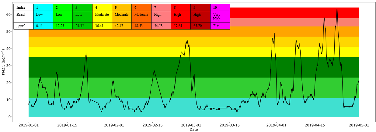
The data used in this study consists of hourly PM2.5 measurements (in µgm-3) from the Eltham monitoring station in the Royal Borough of Greenwich, London. They were extracted from a wider dataset consisting of values from seven different stations over 120 days, from 1st January to 1st May 2019 [21] (Figure 1). Although this figure reveals that air quality is usually low according to the DEFRA PM2.5 banding [22], it also highlights almost weekly PM2.5 peaks that regularly enter the moderate and high pollution levels.

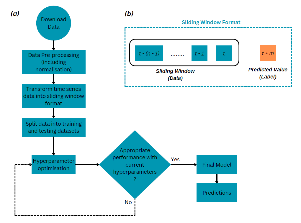
Figure 2 shows the methodology used to develop the models. After following the data preprocessing approach reported in [13], the data were restructured into a sliding window format (Figure 2(b)) before being used for predictions (Figure 2(a)). Then, traditional ML approaches, (i.e., linear regression, RF regression, and XGBoost), and a DL model (i.e., LSTM) were evaluated for forecasting hourly PM2.5 concentration in Eltham. Several sliding window sizes were trialled for each method, starting with 3-hour increments (3 hours, 6 hours, etc), and then narrowing down within ranges of values where the model’s performance was best. A subset of these results is shown in Table 1. Hyperparameter optimisation was carried out for each model using an iterative process as described in Figure 2. The best hyperparameter values for each model at each sliding window length are reported in Table 1.

This study goes much further than [13] and their next hour predictions as it not only investigates predictions for longer horizons from 3 to 24 hours, but also their associated energy consumption. As the size, in hours, of the sliding window is an important performance factor for a given model, values from 3 to 24 hours were investigated. Moreover, the hyperparameters for RF regression, XGBoost and LSTM were optimised using a grid search approach. As per the standards in the field, the root mean squared (RMSE) and mean absolute errors were used to evaluate the models.

Since this work aimed to identify an air quality forecasting method that provides the best performance while using as little energy as possible, the energy usage of both training and prediction processes for each model was calculated. As the CodeCarbon package is well-documented [23], it was chosen to estimate energy consumption in kilowatt-hours (kWh).

3. Results

Table 1 reports performance of the various methods when predicting PM2.5 measurements for the following hour. There, the implementations of RF regression and XGBoost achieve similar results to those reported in [13] and are less performant than both LSTM and LR. Interestingly, one can observe that LR outperformed all other methods, including LSTM, the best method reported by [13]. This may be explained by the fact that, whereas their study considered a much shorter sliding window, i.e., 3 hours, this study explored a wider range of sliding window lengths. Although a 24-hour window was expected to capture potential daily patterns, a 19-hour window proved optimal, possibly by preventing overfitting.

The energy consumption estimations show that LSTM, the deep learning approach, is the most energy-intensive method by far. The best-performing LSTM model consumed 2840 times more energy during training, and 126 times more energy during prediction, than the best-performing LR model (Table 1, Figure 3). Although the other methods are more energy intensive than LR, they are still much more sustainable than LSTM. Indeed, compared to LSTM, the best RF regression and XGBoost models consumed 137 and 278 times less energy during training, and 49 and 13 times less energy during prediction, respectively.

Table 1: Comparative results for 1 hour prediction of traditional machine learning methods and those reported in [11]. Energy ratio is defined by the energy consumption of a model during training or predicting divided by that of the best performing LSTM solution.

Model	Hyperparameters	Sliding window size	MAE	RMSE	Energy ratio (training)	Energy ratio (predicting)
Linear regression	N/A	3 hours	0.239	0.579	1941	88
	N/A	12 hours	0.239	0.581	2951	27
	N/A	19 hours	0.235	0.574	2840	126
	N/A	24 hours	0.237	0.577	1268	31
Random forest	estimators: 40, max_depth: 7	3 hours	0.316	0.583	137	49
	estimators: 45, max_depth: 6	12 hours	0.332	0.603	67	47
	estimators: 20, max_depth:6	24 hours	0.35	0.612	2	2
XGBoost	estimators: 100, max_depth: 4, learning rate: 0.1	3 hours	0.327	0.602	278	13
	estimators: 100, max_depth: 2, learning rate: 0.1	12 hours	0.361	0.623	358	15
	estimators: 95, max_depth: 2, learning rate: 0.1	24 hours	0.372	0.630	79	28
LSTM (optimiser: adam, loss: ‘mae’)	units: 39, learning rate: 0.001, batch size: 24	3 hours	0.487	0.821	1.9	0.2
	units: 42, learning rate: 0.001, batch size: 24	12 hours	0.423	0.684	0.9	0.8
	units: 42, learning rate: 0.001, batch size: 24	19 hours	0.398	0.649	1	1
	units: 45, learning rate: 0.001, batch size: 24	24 hours	0.439	0.710	1.4	0.9
Linear regression [13]	N/A	3 hours	0.333	0.579	/	/
Random forest [13]	Not specified	3 hours	0.331	0.591	/	/
XGBoost [13]	Not specified	3 hours	0.345	0.617	/	/
LSTM [13]	Not specified	3 hours	0.292	0.574	/	/

Table 2: Predictions using linear regression, with a 19-hour sliding window, for a variety of prediction horizon lengths.

 

Prediction Horizon	MAE	RMSE
T + 1	0.235	0.574
T + 3	0.788	1.322
T + 6	1.292	1.997
T + 9	1.584	2.432
T + 12	2.120	3.228
T + 15	2.376	3.613
T + 18	2.673	4.111
T + 21	2.923	4.529
T + 24	3.219	4.981

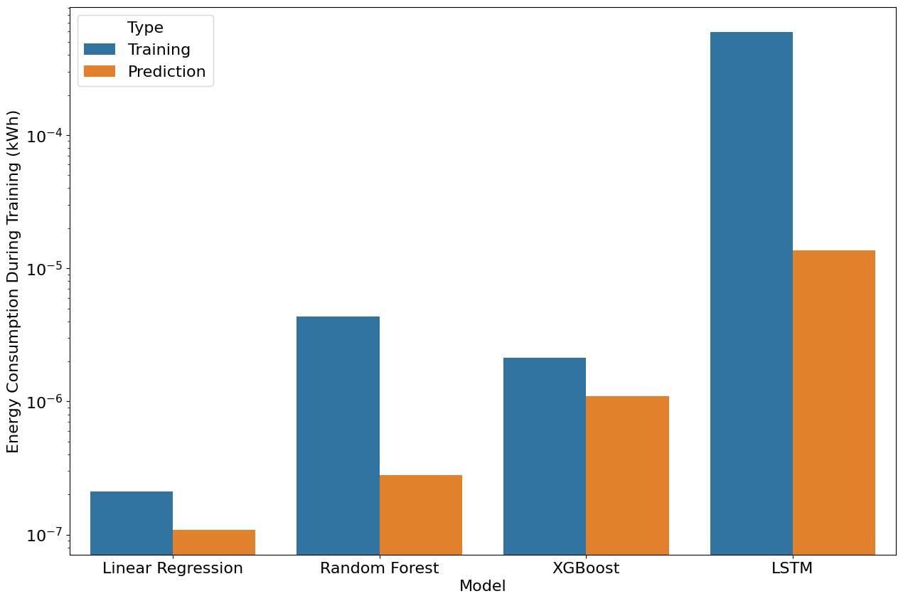
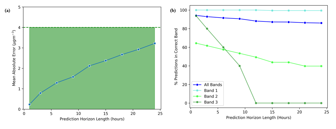
Figure 3 also highlights the difference in energy consumption during training and prediction. For LR and XGBoost, the energy consumption during training was roughly twice that during prediction. However, this figure is 15 times for RF regression, and 44 times for LSTM.

Linear regression also performed well when tested over longer prediction horizons. Table 2 reveals that for this model, MAE and RMSE increase linearly with the length of the prediction horizon within the range of 12 to 24 hours. These MAE values can be compared to the widths of PM2.5 bands used by the UK government to inform public health advice (Figure 1). The narrowest of these bands has a width of 4 µgm^-3, suggesting that predictions up to 24 hours are sufficiently accurate to support decision making (Figure 4(a)). Further analysis shows that over 80% of the model predictions are in the correct band across all prediction horizon lengths. However, one should note that currently the model performs worse for values in higher bands (Figure 4(b)). This can be explained by the fact that, as highlighted on Figure 1, the dataset that was used for this study lacked data points in higher bands, which limited model learning in these areas. Fortunately, this could be remedied by using data collected during a longer period and applying dataset balancing strategies.

Note that in an earlier analysis of this study, preliminary findings were presented at the 2024 World Congress on Civil, Structural, and Environmental Engineering in London, UK [24].

4. Conclusion

Despite the adoption of deep learning solutions in many application areas, this study suggests that linear regression is particularly appropriate to predict air pollution levels in London. Not only does this approach outperform its competitors in terms of MAE and RMSE, but also it consumes the least energy by a significant margin for both training and predicting. In addition, its predictions for a horizon of up to 24 hours are expected to support decision making to reduce particularly harmful human exposure. Although further investigations should be undertaken, this study supports the aspirations that AI-based solutions are sustainable, affordable, and effective, and that their energy needs must be considered during development.

References

[1] F. Godlee, "Air pollution: I-From pea souper to photochemical smog", in BMJ: British Medical Journal, vol. 303, no. 6815, pp. 1459-1461, Dec. 1991. View Article
[2] ML. Bell, DL. Davis, and T. Fletcher, "A retrospective assessment of mortality from the London smog episode of 1952: the role of influenza and pollution", in Environmental Health Perspectives, vol. 112, no. 1, pp. 6-8, Jan. 2004. View Article
[3] P. Brimblecombe, "The Clean Air Act after 50 years", in Weather, vol. 61, no. 11, pp. 311-314, Jan. 2007. View Article
[4] D. Dajnak, D. Evangelopoulos, N. Kitwiroon, S.D. Beevers, and H. Walton, "London health burden of current air pollution and future health benefits of mayoral air quality policies.", in City Hall, pp. 1-72, 2021.
[5] Mayor of London, "Inner London Ultra Low Emission Zone - One Year Report", Feb. 2023. Peer reviewed by Dr G. Fuller, Imperial College.
[6] M. Méndez, M.G. Merayo, and M. Núñez, "Machine learning algorithms to forecast air quality: a survey", in Artificial Intelligence Review, vol. 56, pp. 10031-10066, Feb. 2023. View Article
[7] K. Kumar and B.P. Pande, "Air pollution prediction with machine learning: a case study of Indian cities", in International Journal of Environmental Science and Technology, vol. 20, pp. 5333-5348, May 2023. View Article
[8] M. Castelli, F.M. Clemente, A. Popovič, S. Silva, and L. Vanneschi, "A Machine Learning Approach to Predict Air Quality in California", in Complexity, vol. 2020, Aug. 2020, Art. no. 8049504. View Article
[9] V. Gopalakrishnan. "Hyperlocal air quality prediction using machine learning." Towards Data Science. Accessed: Dec. 19, 2023. [Online] View Article
[10] N.A Zaini, L.W. Ean, A.N. Ahmed, and M.A. Malek, " A systematic literature review of deep learning neural network for time series air quality forecasting", in Environmental Science and Pollution Research, vol. 29, pp. 4958-4990, Jan. 2022. View Article
[11] B. Zhang, Y. Rong, R. Yong, D. Qin, M. Li, G. Zhou, and J. Pan, "Deep learning for air pollutant concentration prediction: A review", in Atmospheric Environment, vol. 290, Dec. 2022, Art. no. 119347. View Article
[12] Y. Li, Z. Sha, A. Tang, K. Goulding, and X. Liu, "The application of machine learning to air pollution research: A bibliometric analysis", in Ecotoxicology and Environmental Safety, vol. 257, Jun. 2023, Art. no. 114911. View Article
[13] A. Utku and U. Can., "Deep Learning Based Air Quality Prediction: A Case Study for London", in Turkish Journal of Nature and Science, vol. 11, no. 4, pp. 126-134, Dec. 2022. View Article
[14] D.A. Wood, "Trend decomposition aids forecasts of air particulate matter (PM2.5) assisted by machine and deep learning without recourse to exogenous data", in Atmospheric Pollution Research, vol. 13, no. 3, Mar. 2022, Art. no. 101352. View Article
[15] P. Henderson, J. Hu, J. Romoff, E. Brunskill, D. Jurafsky, and J. Pineau, "Towards the Systematic Reporting of the Energy and Carbon Footprints of Machine Learning", in The Journal of Machine Learning Research, vol. 21, no. 248, pp. 1-43, 2020.
[16] L. Bouza, A. Bugeau, and L. Lannelongue, "How to estimate carbon footprint when training deep learning models? A guide and review" in Environmental Research Communications, vol. 5, no. 11, Nov. 2023, Art. no. 115014. View Article
[17] A.S. Luccioni, S. Viguier, and A.L. Ligozat, "Estimating the Carbon Footprint of BLOOM, a 176B Parameter Language Model", in The Journal of Machine Learning Research, vol. 24, no. 253, pp. 1-15, 2023.
[18] A. Mehonic and A.J. Kenyon, "Brain-inspired computing needs a master plan", in Nature, vol. 604, pp. 255-260, Apr. 2022. View Article
[19] R. Toews. "Deep Learning's Carbon Emissions Problem". Forbes. Accessed: Dec. 19, 2023. [Online] https://www.forbes.com/sites/robtoews/2020/06/17/deep-learnings-climate-change-problem/?sh=4479178c6b43
[20] J. Rentschler and N. Leonova, "Air Pollution and Poverty: PM2.5 Exposure in 211 Countries and Territories", Policy Research Working Paper in World Bank, Washington, D.C.
[21] S. Nobell. "Pollution PM2.5 data London 2019 Jan to Apr". Kaggle. Accessed: Dec. 19, 2023. [Online] View Article
[22] Department for Environment Food & Rural Affairs (DEFRA). "What is the Daily Air Quality Index?". UK AIR. Accessed: May 7, 2024. [Online] View Article
[23] CodeCarbon. "CodeCarbon - CodeCarbon 2.3.2 Documentation". GitHub. Accessed: Dec. 15, 2023. [Online] View Article
[24] M. Hegde, J.-C. Nebel, and F. Rahman, "Sustainable AI-Based Prediction of Air Pollution Levels in London," in Proc. World Congress on Civil, Structural, and Environmental Engineering, London, UK, April 2024, Art. no. 151. View Article