International Journal of Environmental Pollution and Remediation (IJEPR)
ISSN: 1929-2732

Volume 11 - Year 2023 - Pages 10-19
DOI: 10.11159/ijepr.2023.002
Machine Learning for the Estimation of COD from UV-Vis Spectrometer in Leather Industries Wastewater
Marco Cardia 1, Stefano Chessa1, Massimiliano Franceschi2, Francesca Gambineri2, Alessio Micheli1
1
Department of Computer Science, University of Pisa
Largo Bruno Pontecorvo 3, 56125, Pisa, Italy
marco.cardia@phd.unipi.it; stefano.chessa@unipi.it, alessio.micheli@unipi.it
2Archa S.R.L.
Via di Tegulaia 10/A, 56121, Ospedaletto, Pisa, Italy
massimiliano.franceschi@archa.it, francesca.gambineri@archa.it
Abstract - In this paper, we introduce a method for analysing wastewater from the leather industry with a specific focus on determining the Chemical Oxygen Demand parameter, which plays a vital role in evaluating water pollution levels. Conventional methods for measuring it involve extensive laboratory analysis, sample preparation, and the usage of hazardous substances. To overcome these limitations, we propose a machine learning-based approach that employs nonspecific sensors and soft sensing techniques to derive indicators of wastewater quality. Our method leverages ultraviolet and visible spectroscopy measurements, which provide valuable insights into the light absorption characteristics of the wastewater sample, enabling us to estimate Chemical Oxygen Demand. Importantly, our approach includes an analysis of the input wavelengths, allowing us to identify the spectra for accurate Chemical Oxygen Demand estimation. Once deployed, our method offers the potential for real-time monitoring systems of wastewater in leather production contexts, by eliminating the need for time-consuming laboratory analyses.
Keywords: Machine Learning, Industry 4.0, Soft Sensing, Wastewater, Chemical Oxygen Demand, Leather Industry.
© Copyright 2023 Authors - This is an Open Access article published under the Creative Commons Attribution License terms. Unrestricted use, distribution, and reproduction in any medium are permitted, provided the original work is properly cited.
Date Received: 2023-05-13
Date Revised: 2023-06-18
Date Accepted: 2023-06-29
Date Published: 2023-07-05
1. Introduction
The leather industry is highly water intensive and has an important environmental impact. Water is employed as a medium to convert raw hides and skin into leather. In most cases, wastewater produced by the processes in the leather industry is dangerous to the environment. Tannery wastes are characterised by high Biochemical Oxygen Demand (BOD), high Chemical Oxygen Demand (COD), high pH, high chromium, and high dissolved salts. Chromium is widely used in chrome tanning processes [1]. Discharging contaminated effluent into a receiving water body could spread diseases to human beings [2]–[5]. In a case study of the groundwater quality around leather industries in South India is reported a high level of pollution around the tanneries [1]. This fact suggests the importance of studying new ways of analysing water quality in wastewater generated by leather industries. In Italy, in particular, in Tuscany, wastewater coming from tanneries is treated by external Wastewater Treatment Plants. Here, dangerous compounds are replaced with environmentally safe fluids waste and solid waste. Some parameters used to establish if a leather industry is complying with certain limits are pH, Total Suspended Solids (TSS), COD, BOD, total chlorides, total sulphates, ammonia, and chromium. The same parameters are also used by Wastewater Treatment Plants to establish the charge that a tannery should pay. Similarly, the European Union uses these measures to define certain objectives that each member state has to achieve to satisfy specific water quality standards. The guidelines are published in 2001 by the European Co-operation in the field of Scientific and Technical research (COST) and refer to the constraints the effluent of Wastewater Treatment Plants has to satisfy [6], [7].
The COD is defined as the quantity of oxygen required to oxide the organic component of a water sample using a strong oxidising agent, such as dichromate [8]. It is expressed in milligrams per litre (mg/l), which is the mass of oxygen consumed for a litre of solution. It is considered one of the most important parameters to evaluate the degree of pollution of wastewater by the Association of Analytical Chemists [9]. Currently, the method used to measure COD in wastewater is titration, which involves the usage of a strong chemical oxidant [10]. Among others, the most commonly used oxidant is potassium dichromate, in combination with sulphuric acid. This method is the standard method to measure COD according to the American Public Health Association (APHA) [7].
However, the conventional method has some drawbacks: it requires a long time in order to obtain the result and it requires manual operations. Furthermore, the chemicals used to make the reactions are dangerous for the environment. There are alternatives to the titrimetric analysis, such as the colorimetric measurement. Even if it is considered faster and easier to perform, it still needs the usage of dangerous chemicals [11], [12]. During the last decades, standard methods for chemical measuring have been aided by a new technique named chemometrics, a data-driven approach which allows the extraction of information from chemical systems [13]. However, only in the last years’ real chemometrics applications have become feasible, thanks to the large availability of sensors. A possible application of chemometrics is through soft-sensing. A soft sensor allows obtaining a particular measure from nonspecific sensors. Soft-sensing is particularly useful when some relevant product qualities or quantities are difficult to be measured due to technical or economic issues. In the context of chemometrics, the usage of the soft-sensing technique allows for obtaining water quality parameters, such as COD or BOD, in a manner of seconds instead of hours using nonspecific sensors. In this way, the usage of toxic, corrosive and dangerous reagents is avoided.
In this paper, we propose an automatic data analysis approach for the analysis of wastewater. The proposed method, built over our preliminary work [14], leverages soft sensing and machine learning, allowing the determination of a water quality indicator using nonspecific sensors. In particular, the method can determine the COD by exploiting an optical sensor (a spectrophotometer), using the ultraviolet and visible (UV-Vis) wavelengths. To build the soft sensor different machine learning models have been compared. Moreover, we integrate the previous work providing an analysis of the wavelengths exploited by the model to estimate the COD. Data used to train the models are provided by ARCHA S.R.L.1 , a chemical laboratory located in Pisa, Italy. The dataset used for our experiments contains samples from three tanneries that refer to fourteen distinct stages of the leather production process. We run experiments exploiting machine learning models with different preprocessing settings. We compute the logarithmic COD to obtain a normal distribution of data, we reduce the dimensionality of the input through the Principal Component Analysis and we train machine learning models to find a correlation between the sensor data and the COD. We compare Multilinear Regression Model, Random Forest, Support Vector Regressor, K-Nearest Neighbours and Multilayer Perceptron. The validation is made through a double K-Fold Cross-Validation. We use the coefficient of determination, Root Mean Squared Error, and Average Absolute Relative Error as evaluation metrics to compare the performances of the different models. According to our results, the Multilayer Perceptron provides better estimation than other models. It can be observed that, after the model training, our approach does not require any (time-expensive) laboratory analyses. These results open to the use of nonspecific sensors, that do not require the use of dangerous chemicals and complex workflows, in the context of real-time monitoring of wastewater of leather industries.
2. Related Work
As stated by the American Public Health Association (APHA), the standard method for determining COD is the dichromate method with the use of potassium dichromate [7]. This conventional method has some drawbacks, such as being time-consuming, the usage of a strong oxidant, and troublesome manual operations.
During the last years the application of chemometrics, i.e. the usage of data-driven models for extracting information from chemical systems, is increasing thanks to the large availability of sensors and Beer-Lambert's law [15]. It states that there is a correlation between the absorption spectrum and the concentration of a certain substance [15]. Different pollutants have different absorption characteristics. Therefore, by exploiting Beer-Lambert's law it is possible, based on a theoretical basis, to extract the concentration of pollutants in water. However, a linear relationship needs strict requirements and it is difficult to obtain. Indeed, the effluents often contain mixed chemicals, and it is difficult to detect all the components simultaneously through the absorption spectrum. For this reason, machine learning models, able to detect complex non-linear relationships, are largely adopted [16].
To the best of our knowledge, this is the very first study for COD estimation in the context of leather industry wastewater. Related works can be found, but they are related to Wastewater Treatment Plants and not directly applied to the estimation of COD in wastewater coming from the different processes involved in leather production. Most of the works found in the literature exploit Multi-linear Regression to provide COD estimation from spectroscopy [17]–[20]. Others used Artificial Neural Networks as a machine learning model to find the correlation between the absorption spectrum and COD [19], [21]. Every author but one used the UV-Vis spectrum as input for the model [17], [19], [21], the other one compared the UV-Vis spectrum with the Near Infrared (NIR) wavelengths [20]. First solutions adopted a single wavelength for the estimation of the COD [22], however, the complexity of the wastewater, particularly in the context of industrial wastewater, makes it difficult to find a correlation using a single or few wavelengths.
Alam developed a method based on UV-Vis spectrometry for the determination of COD in a Wastewater Treatment Plant [17]. His method consists in building a linear regression model able to the most sensitive wavelengths using a 10 nm bandwidth at different wavelengths and correlating them with the COD measurement. The spectrophotometer used by the author was able to detect absorbance values from wavelengths starting from 180 nm to 900 nm with a 20 nm step size [17].
Chen et al. used the soft-sensor technique to determine three different measures related to water quality, i.e. the nitrate, the COD and the turbidity [18]. They exploited the UV-Vis absorption spectrometry together with the analysis of the wavelengths in order to estimate the nitrate, the COD and the turbidity simultaneously [18]. According to the measure they would like to estimate, they leverage different wavelengths. A set of wavelengths were first provided to a Partial Least squares Regression (PLSR) model in order to obtain the estimated turbidity. On the other hand, to establish the approximation of the COD, the input to the PLSR model was previously preprocessed by the Multiplicative Scatter Correction (MSC) method, which removed the turbidity interference. To provide the estimation of the Nitrate, the spectral difference between the COD spectrum and the turbidity-compensated spectrum was performed. The absorption spectrum, after the COD compensation, was selected and the nitrate concentration has been obtained after applying the PLSR algorithm [18].
Fogelman et al. exploited a Multilayer Perceptron (MLP) to build a soft-sensor able to estimate COD values for wastewater samples [19]. They extracted a limited number of features from the full spectrum of wastewater samples obtained through ultraviolet (UV) spectroscopy. Then, using the key features of the spectral absorbance pattern, they trained an MLP. They validate the model by comparing the results of their MLP against a traditional Multiple Linear Regression (MLR) [19].
Charef et al. presented a soft sensor used to extract the concentration of COD from the UV spectrum, temperature, pH, and conductivity [21]. In the preprocessing phase, they selected the most relevant variables using the Principal Component Analysis. Then, the selected 15 variables are used to train a Multilayer Perceptron that provides the estimated COD [21]. However, their results are related to a wastewater treatment plant, which in general has lower values of COD. Thus, their results are not comparable to ours.
Sarraguça et al. compared two methods for the determination of three water quality parameters, namely COD, Nitrate concentration, and TSS [20]. The first method exploits the UV-Vis spectrum, while the second one leverage the NIR spectrum. In both cases, a preprocessing phase was performed to select the most relevant wavelengths through the bootstrap method. The selected wavelengths were used to train a Partial Least Squared Regression model [20]. Also in this case their results refer to a wastewater treatment plant and are not comparable to ours.
3. Methodology
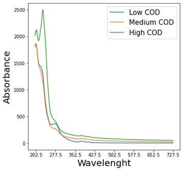
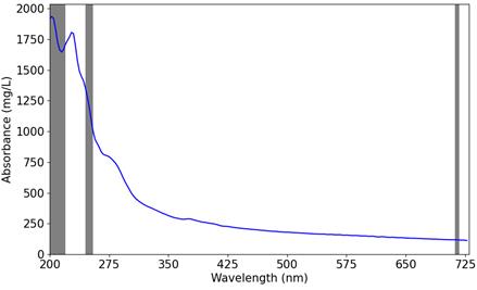
For the purpose of training and validation of our machine learning models for the estimation of COD, we collected a dataset of 151 samples using a UV-Vis spectrophotometer in three tanneries, and each sample refers to a specific phase of the leather production process. The spectrophotometer provides the absorbance value for different wavelengths, in the UV and Visible spectrum, from 200 nm to 730 nm with intervals of 2.5 nm (hence, each sample report information about 212 different wavelengths). An example of three different measurements of the absorption spectrum is provided in Figure 1.
Each sample is associated with its ground truth, its COD, as it is measured in ARCHA. Other metadata for each sample are the phase and the leather industry. ARCHA provided three incremental releases of the dataset. The first version contains 89 samples, the second one has 119 samples, and the last has 151 samples. Each sample is a vector in a 212-dimensional space. In this context, where the number of samples is lower than the dimension of the space, we may incur the curse of dimensionality [23]. It indicates that the number of samples necessary to estimate an arbitrary function grows exponentially with respect to the dimensionality of the function itself. Hughes studied the behaviour of the predictive power of a model, fixing the dataset size and varying the size of the dimensions. As the dimension increases, the performance improves up to a certain dimension, after which the performance deteriorates [24].
Since our dataset has 151 samples spread over 212 dimensions, and because of this it may be too "sparse" for our purposes, we tested two techniques for dimensionality reduction: (i) a "naive" solution that consists in selecting the k absorbance wavelengths with the highest variance (hereafter k-AV), and (ii) the Principal Component Analysis (PCA) using the singular value decomposition. As will be discussed in more detail in Section 4, since the ground truth has a positive skew distribution, we use its logarithm in our experiments. Although estimating the COD from a spectrophotometer sample is a regression task, which is known to be insensitive to standardisation and normalisation, we use anyway the standardization of the dataset as it improves the stability and the convergence of the algorithms [25].
Due to the lack of availability of public benchmarks, it is not possible to compare our results against other works in the literature. For this reason, we focus this work on the comparison of five different machine learning models, namely linear regressor, random forest, Support Vector Regressor (SVR), K-Nearest Neighbours (KNN), and Multilayer Perceptron (MLP). To ensure the robustness and the generalisability of our result, we use a double 5-fold cross-validation to evaluate the performance of our models. In this approach, the data are first split into k folds, and then an inner k-fold cross-validation is performed on each of the external k folds. The outer loop is used to assess the performance of the model (test set), while the inner loop is used to optimise the model’s hyperparameters. This allows us to evaluate the models’ performance on new data (with a test set comprising the entire dataset) that was not used either to train or to optimise their hyperparameters and provides a more reliable estimation of their performance compared to a standard hold-out approach. We select the hyperparameters by launching a grid search for all the models except the MLP, for which we use a random search over the hyperparameter space.
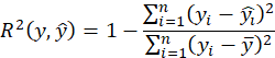
We evaluate our models using the coefficient of determination, the Root Mean Squared Error and the Average Absolute Relative Error metrics. The coefficient of determination (also known as R2 score) is a statistical measure that explains the variation of one dependent variable that is predictable from the independent variables. A score of 1.0 us the best possible score. Its value can be negative because the model can be arbitrarily worse. As an example, a model that always provide the expected value of y as estimation, without considering the input features, has a R2 value of 0. If (yi ) ̂ is the predicted value of the i-th sample and yi is the corresponding true value for total n samples, the estimated coefficient of determination R2 is defined as:
where
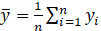 , and
, and 
The Root Mean Squared Error (RMSE) is the average squared difference between an estimated and the actual value. It is used as a measure of the quality of an estimator. It is always positive and as it decreases, the better the model. It can be obtained as:
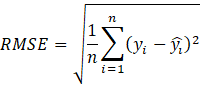
where yi is the actual value, ![]() ̂is the estimated one and n is the number of samples.
̂is the estimated one and n is the number of samples.
The Average Absolute Relative Error (AARE) provides the performance index in terms of the predicting measure and the distribution of the prediction error. It is defined as:

Where ti represents the observed measure for the i-th sample, pi is the estimated measure for the i-th sample, N is the total number of samples. The smaller is the AARE value, the better the performance.
4. Experiments
The difficulty of the estimation of the COD of wastewater using the absorbance from a single or few wavelengths lies in the fact that wastewater is made up of multi-components. Indeed, industrial wastewater, in particular in the case of tanneries, contain high pollution characteristics such as suspended solids and high concentration of chloride, ammonia, and chromium [1], [26]–[28], which are implicitly estimated in terms of COD, TSS, electrical conductivity and pH indexes.
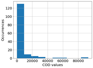
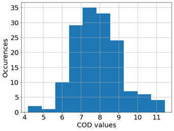
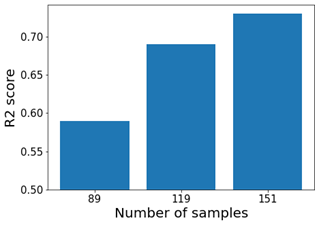
In our dataset, the distribution of the COD values is strongly positively skewed, as shown in Figure 2. It is possible to observe that most of the samples have a COD below 10000 mg/l. In order to obtain a better distribution of data with respect to the COD, we used its logarithm in the training of our models, which, as shown in Figure 3, has a Gaussian-like distribution. This transformation reduces the skewness of the data and makes it more symmetrical. In experiments performed with and without this transformation, we observe that the performances of the models are improved by taking the logarithmic COD values, for example, the MLP performance increases from 0.64 to 0.68 in the R^2 metric. For some models this transformation allows them to align with their assumption: for example, the linear regression assumes that the data follows a Gaussian distribution. While the transformation of the target variable improved the performance of the models, we also need to consider the size of the dataset. Figure 4 shows the results of the machine learning model having the best performance in terms of R2 in the different releases of the dataset. Here, it is possible to observe how the increment in the number of samples leads to better model performance.
In all three releases of the dataset, we observe the strongly positive skewness of the COD values. The first version contained 89 samples. The COD values ranged from 66 mg/L to 19200 mg/L. The second one contained 119 samples, the COD values ranged from 66 mg/L to 92900 mg/L. The last release contains 151 samples and the COD values range from 66 mg/L to 92900 mg/L. Note that the periodical upgrade of the dataset is required by the long time necessary to collect samples, in particular, to extract the COD through laboratory analysis.
Indeed, the estimation of the COD from the conventional methods is a time-hungry operation. Since the processes in the leather industry involve the usage of different chemicals in different quantities that could increase the COD value, the experiments conducted with the last release of the dataset, consider also the process. To represent this categorical variable, we exploit the one-hot representation. With respect to the trials that do not use this variable, we observe an increment in the R^2 (from 0.71 to 0.73) and the reduction of the RMSE (from 9393 mg/l to 8563 mg/l). For this reason, we consider the phase an important variable for COD estimation. The final configuration, after the preliminary results, for the final results is a 29-dimensional vector X∈R29, where 15 are the absorbances extracted by the PCA and the last 14 are the one-hot encoding representation of the 14 phases. Experiments are conducted using the scikit learn and the PyTorch libraries.
Hereafter, we provide a list of the machine learning models used to estimate the COD, along with their respective hyperparameters. Additionally, we include the relative range of values and the number of sampled values in that range (# values). They refer to the values used for the model selection phase using the Grid Search.
- Linear model
Table 1. Hyperparameters and values for the Linear model. α is the coefficient for Tikhonov regularization.
|
|
Range |
# values |
|
α |
[1x10-15, 1x10¹⁰] |
20 |
- Random Forest
Table 2. Hyperparameters and values for the Random Forest model. max_depth is the maximum depth of the tree. min_samples_leaf is the number of samples required to be at a leaf node. min_samples_split is the minimum number of samples required to split an internal node. n_estimators is the number of tress in the forest. criterion is the function used to measure the quality of the split.
|
|
Range |
# values |
|
n_estimators |
[10, 50] |
5 |
|
max_depth |
[1, 20] |
20 |
|
min_samples_leaf |
[1,30] |
5 |
|
min_samples_split |
[2,30] |
5 |
|
|
Values |
|
criterion |
[poisson, friedman_mse, squared_error, absolute_error] |
- Support Vector Regressor (Gaussian Kernel)
Table 3. Hyperparameters and values for the SVM model. C is the regularisation parameter. γ is the radius of the kernel for the support vectors. ε is the size of the margin for which no penalty is given to errors.
|
|
Range |
# values |
|
C |
[1x10⁻¹⁰, 1x10³] |
10 |
|
γ |
[1x10⁻¹⁰, 1x10³] |
10 |
|
ε |
[0.05, 0.5] |
5 |
- K-Nearest Neighbours
Table 4. Hyperparameters and values for the KNN model. K is the number of samples exploited to make a prediction. metric is the function used to calculate the distance between the data points.
|
|
Range |
# values |
|
K |
[1, 30] |
10 |
|
|
Values |
|
metric |
[euclidean, minkowki, manhattan] |
- Multilayer Perceptron (MLP)
Table 5. Hyperparameters and values for the MLP model. learning rate is the step size to update the MLP’s parameter. units is the number of units of the hidden layer. momentum controls the influence of previous parameter updates during the training. weight decay is the regularization parameter. act_fun is the non-linear function applied to the output of a unit in a MLP.
|
|
Range |
# values |
|
learning rate |
[1x10⁻⁵, 1x10⁻²] |
10 |
|
units |
[20, 800] |
10 |
|
momentum |
[0],[0.6, 0.9] |
5 |
|
weight_decay |
[0, 0.3] |
5 |
|
|
Values |
|
act_fun |
[Sigmoid, Tanh, ReLU] |
5. Results
We compared the performance of 5 machine learning models on the dataset provided by ARCHA relatives to different tanneries in Italy. Table 6 contains the results in the training, validation and test set for the RMSE, and in both the training and test sets for R2 and AARE. The reported test results refer to the average of five different iterations, belonging to the outer set from the double 5-fold cross-validation technique. Moreover, the table contains the standard deviation in the format (±std) for R2 and AARE.
The null model is an estimator which always provides as estimation the average of the COD of the training set. It is used as a baseline. It is possible to observe that all the models have significantly better performance with respect to the baseline, i.e. the null model. The model having the best performance is the MLP both in terms of RMSE and R2. The SVR with a Radial Basis Function (RBF) kernel outperforms the other models in terms of AARE. However, all the models with non-linear capabilities have similar performances, with a R2 higher than 0.70 in the test set. On the other hand, the linear regressor has lower performance due to the incapability to include nonlinear relationships. We have to consider that collected data come from a context where the wastewater is highly polluted. They are relative to different processes, each characterised by the usage of different chemical agents and the presence of suspended solids. The concentration of the chemical species affects the absorbance: higher concentrations result in stronger absorbance signals [16]. Indeed, involving the process in the estimation of COD allows us to obtain a more reliable estimation, since each process exploits different chemicals, even if the samples for each process are poor (a mean of around 10 samples for each process). Due to these considerations, the current results satisfy the expectation of ARCHA experts.
Table 6: Results of different machine learning models for the estimation of COD.
|
Model |
RMSE |
RMSE validation (mg/l) |
RMSE |
R2 training |
R2 |
AARE training |
AARE test |
|
Null model |
14484.63 |
14093.06 |
14165.22 |
0 (±0) |
-0.01 (±0) |
15.44% (±0.24%) |
17.14% (±0.94%) |
|
Linear regressor |
5754.54 |
8684.29 |
13638.93 |
0.81 (±0.08) |
0.63 (±0.10) |
6.40% (±0.89%) |
8.14% (±0.87%) |
|
Random forest |
6529.55 |
8300.26 |
9768.54 |
0.91 (±0.07) |
0.70 (±0.08) |
3.43% (±0.71%) |
7.08% (±0.59%) |
|
SVR (RBF kernel) |
3619.32 |
8215.56 |
9604.72 |
0.81 (±0.07) |
0.71 (±0.08) |
3.95% (±0.87%) |
6.26% (±1.13%) |
|
KNN |
9082.29 |
8579.17 |
9192.89 |
0.81 (±0.07) |
0.71 (±0.07) |
5.24% (±0.47%) |
7.02% (±0.53%) |
|
MLP |
4487.51 |
6833.72 |
8563.10 |
0.93 (±0.08) |
0.73 (±0.10) |
3.11% (±0.54%) |
7.65% (±0.70%) |
6. Model interpretation and discussion
Ultraviolet (UV) - Visible (Vis) spectroscopy is a technique used to measure the absorption of light by matter. The main difference between the UV and Vis spectroscopy is the wavelength range of light that they measure. UV spectroscopy measures the absorption of ultraviolet light, which has a shorter wavelength and higher energy than visible light. Vis spectroscopy, on the other hand, measures the absorption of visible light, which has a longer wavelength and lower energy than ultraviolet light. [29]
The measurement of Chemical Oxygen Demand (COD), which quantifies the concentration of organic compounds in water, can be facilitated through the utilization of UV spectroscopy. This is because organic compounds in water have the ability to absorb UV light, and the degree of absorption is directly related to the concentration of these compounds within the water sample. However, it is crucial to acknowledge that wastewater samples can potentially contain multiple absorbing species. Moreover, the presence of turbidity in the wastewater sample may significantly influence the accuracy of measurements.
It is important to note that the absorbance observed within the long wavelength visible range (440 nm to 800 nm) can be attributed to turbidity or to coloured compounds that absorb at visible spectrum. The presence of these in the sample can complicate the determination of organic compound concentrations.
In order to provide an explanation of the model's behaviour, it is necessary to consider the specific wavelengths used for its predictions. To achieve this, we leverage the random forest model, which enables the determination of the most relevant features. Figure 5 showcases the most important wavelengths used to estimate the COD by the random forest model. The presented signal represents the mean of the dataset signals. The model focuses on the UV wavelengths range spanning from 200 nm to 225 nm, as well as around 254 nm and around the 720 nm spectrum. The importance attributed by the model to these wavelengths aligns with the absorption characteristics of wastewater and the expert opinions. This analysis highlights the reliability of the model’s estimation, as its predictions are based on wavelengths where organic compounds absorb light. Additionally, the focus of the model around the 720 nm wavelength is justified by the possible presence of turbidity and coloured compounds.
7. Conclusion
This work presents a novel soft sensor to estimate the COD of leather industrial wastewaters, that leverages a UV-Vis spectrophotometer and machine learning models. For the purpose of its development, we considered and compared different machine learning models that correlate the acquired spectra with the monitored parameter (COD). Specifically, we consider linear model, random forest, SVR, KNN, and MLP. The obtained results show that the MLP performs better than other models. However, all the selected models are able to estimate the COD with good performances. Our experiments also show the importance of the number of samples, and the importance of the dimensionality reduction. Moreover, we provide an analysis of the predictions provided by the Random Forest. These are based on specific wavelengths that are in accordance with ARCHA experts.
Future works will focus on the enlargement of the dataset, also through data augmentation techniques. In this way, it would be possible to train a model also on a single phase of the leather production process. We will also train a new model able to analyse the trend of the signal, exploiting Convolutional Neural Networks and Recurrent Neural Networks. Moreover, we will also focus on the problem of estimation of other water quality parameters such as the Total Suspended Solids (TSS) and the Biochemical Oxygen Demand (BOD). Beyond this, we plan to validate our soft sensor in some leather production plants, with the purpose of extending the dataset and of analysing in real-time the level of pollutants in the different production phases, with the purpose of identifying best practices in the production.
References
[1] P. J. Sajil Kumar and E. J. James, "Assessing the Impact of Leather Industries on Groundwater Quality of Vellore District in South India Using a Geochemical Mixing Model," Environmental Claims Journal, vol. 31, no. 4, pp. 335-348, Oct. 2019, doi: 10.1080/10406026.2019.1622864. View Article
[2] M. M. Hamed, M. G. Khalafallah, and E. A. Hassanien, "Prediction of wastewater treatment plant performance using artificial neural networks," Environmental Modelling & Software, vol. 19, no. 10, pp. 919-928, Oct. 2004, doi: 10.1016/j.envsoft.2003.10.005. View Article
[3] F. S. Mjalli, S. Al-Asheh, and H. E. Alfadala, "Use of artificial neural network black-box modeling for the prediction of wastewater treatment plants performance," J Environ Manage, vol. 83, no. 3, pp. 329-338, May 2007, doi: 10.1016/J.JENVMAN.2006.03.004. View Article
[4] S. Naidoo and A. O. Olaniran, "Treated Wastewater Effluent as a Source of Microbial Pollution of Surface Water Resources," OPEN ACCESS Int. J. Environ. Res. Public Health, vol. 11, p. 11, 1990, doi: 10.3390/ijerph110100249. View Article
[5] "Health guidelines for the use of wastewater in agriculture and aquaculture. Report of a WHO Scientific Group.," World Health Organ Tech Rep Ser, vol. 778, 1989.
[6] J. B. Copp, "The COST Simulation Benchmark: Description and Simulator Manual (a product of COST Action 624 & COST Action 682)," 2001.
[7] E. Rice, R. Baird, A. Eaton, and L. Clesceri, "Standard Methods for the Examination of Water and Wastewater," Standard Methods, 2012.
[8] ISO, "Water Quality-Determination of the chemical oxygen demand," in International Standard, 1986.
[9] W. Horwitz, P. Chichilo, and H. Reynolds, "Official methods of analysis of the Association of Official Analytical Chemists," Official methods of analysis of the Association of Official Analytical Chemists., 1970.
[10] W. Allan Moore, R. C. Kroner, and C. C. Ruchhoft, "Dichromate Reflux Method for Determination of Oxygen Consumed," Anal Chem, vol. 21, no. 8, 1949, doi: 10.1021/ac60032a020. View Article
[11] A. M. Jirka and M. J. Carter, "Micro semiautomated analysis of surface and waste waters for chemical oxygen demand," Anal Chem, vol. 47, no. 8, pp. 1397-1402, Jul. 1975, doi: 10.1021/ac60358a004. View Article
[12] T. M. Lapara, J. E. Alleman, and P. G. Pope, "Miniaturized closed reflux, colorimetric method for the determination of chemical oxygen demand," Waste Management, vol. 20, no. 4, 2000, doi: 10.1016/S0956-053X(99)00304-9. View Article
[13] S. Wold, "Chemometrics; what do we mean with it, and what do we want from it?," Chemometrics and Intelligent Laboratory Systems, vol. 30, no. 1, 1995, doi: 10.1016/0169-7439(95)00042-9. View Article
[14] M. Cardia, S. Chessa, M. Franceschi, F. Gambineri, and A. Micheli, "Estimation of COD from UV-Vis Spectrometer Exploiting Machine Learning in Leather Industries Wastewater," in Proceedings of the 8th World Congress on Civil, Structural, and Environmental Engineering, Lisbon, Portugal, 2023. doi: 10.11159/iceptp23.160. View Article
[15] D. F. Swinehart, "The Beer-Lambert law," Journal of Chemical Education, vol. 39, no. 7. 1962. doi: 10.1021/ed039p333. View Article
[16] W. Hu, "The application of artificial neural network in wastewater treatment," in 2011 IEEE 3rd International Conference on Communication Software and Networks, ICCSN 2011, 2011, pp. 338-341. doi: 10.1109/ICCSN.2011.6013606. View Article
[17] T. Alam, "Estimation of Chemical Oxygen Demand in WasteWater using UV-VIS Spectroscopy," 2010.
[18] X. Chen, G. Yin, N. Zhao, T. Gan, R. Yang, M. Xia, C. Feng, Y. Chen, Y. Huang, "Simultaneous determination of nitrate, chemical oxygen demand and turbidity in water based on UV-Vis absorption spectrometry combined with interval analysis," Spectrochim Acta A Mol Biomol Spectrosc, vol. 244, p. 118827, Jan. 2021, doi: 10.1016/j.saa.2020.118827. View Article
[19] S. Fogelman, M. Blumenstein, and H. Zhao, "Estimation of chemical oxygen demand by ultraviolet spectroscopic profiling and artificial neural networks," Neural Comput Appl, vol. 15, no. 3-4, pp. 197-203, Jun. 2006, doi: 10.1007/s00521-005-0015-9. View Article
[20] M. C. Sarraguça, A. Paulo, M. M. Alves, A. M. A. Dias, J. A. Lopes, and E. C. Ferreira, "Quantitative monitoring of an activated sludge reactor using on-line UV-visible and near-infrared spectroscopy," Anal Bioanal Chem, vol. 395, no. 4, pp. 1159-1166, Oct. 2009, doi: 10.1007/s00216-009-3042-z. View Article
[21] A. Charef, A. Ghauch, P. Baussand, and M. Martin-Bouyer, "Water quality monitoring using a smart sensing system," Measurement (Lond), vol. 28, no. 3, pp. 219-224, Oct. 2000, doi: 10.1016/S0263-2241(00)00015-4. View Article
[22] H. Kong and H. Wu, "A Rapid Determination Method of Chemical Oxygen Demand in Printing and Dyeing Wastewater Using Ultraviolet Spectroscopy," Water Environment Research, vol. 81, no. 11, 2009, doi: 10.2175/106143009x426059. View Article
[23] B. Richard Bellman and R. Kalaba, "A mathematical theory of adaptive control processes," Proceedings of the National Academy of Sciences, vol. 45, no. 8, pp. 1288-1290, Aug. 1959, doi: 10.1073/PNAS.45.8.1288. View Article
[24] G. F. Hughes, "On the Mean Accuracy of Statistical Pattern Recognizers," IEEE Trans Inf Theory, vol. 14, no. 1, pp. 55-63, 1968, doi: 10.1109/TIT.1968.1054102. View Article
[25] M. S. Shanker, M. Y. Hu, and M. S. Hung, "Effect of data standardization on neural network training," Omega (Westport), vol. 24, no. 4, pp. 385-397, Aug. 1996, doi: 10.1016/0305-0483(96)00010-2. View Article
[26] H. Sawalha, R. Alsharabaty, S. Sarsour, and M. Al-Jabari, "Wastewater from leather tanning and processing in Palestine: Characterization and management aspects," J Environ Manage, vol. 251, Dec. 2019, doi: 10.1016/J.JENVMAN.2019.109596. View Article
[27] T. Admassu, A. Desta, and F. Assefa, "Assessment of the physico-chemical characteristics of a tannery wastewater and its pollution impact on the water quality of Little Akaki River," Ethiopian Journal of Biological Sciences, vol. 18, no. 1, pp. 77-94, Nov. 2020, Accessed: Nov. 25, 2022. [Online]. Available: https://www.ajol.info/index.php/ejbs/article/view/201469
[28] A. Rajeswari, "Efficiency of effluent treatment plant and assessment of water quality parameters in tannery wastes," Pelagia Research Library European Journal of Experimental Biology, vol. 5, no. 8, pp. 49-55, 2015, Accessed: Nov. 25, 2022. [Online]. Available: www.pelagiaresearchlibrary.com
[29] G. Kaur, H. Singh, and J. Singh, "UV-vis spectrophotometry for environmental and industrial analysis," Green Sustainable Process for Chemical and Environmental Engineering and Science: Analytical Techniques for Environmental and Industrial Analysis, pp. 49-68, Jan. 2021, doi: 10.1016/B978-0-12-821883-9.00004-7. View Article