International Journal of Environmental Pollution and Remediation (IJEPR)

ISSN: 1929-2732

1. Introduction

Ozone (O₃), is a secondary air pollutant [30], acts as a strong oxidizing agent in the lower atmosphere (troposphere) [1], generated through chemical reactions involving oxides of nitrogen (NO_x) and volatile organic compounds (VOCs) [2]. The rapid pace of urbanization has exposed many individuals to elevated O₃ levels, increasing the risk of both immediate and long-term health consequences [3]. Numerous epidemiological studies have explored a connection between ozone concentrations and hospital admissions for a range of medical ailments such as pregnancy complications [4], conjunctivitis [5], influenza [6], mortality risks [7] including various respiratory issues [8]. The road traffic emerges as the predominant source of emissions for photochemical precursors like NO_x and VOCs [9]. O₃ concentration is dependent on the NO/NO₂ ratio and VOC-sensitivity. O₃ photochemical system (O₃-NO_x-VOC chemistry) is very complex mechanism in the open atmosphere system [31].

In India, road transportation predominantly relies on diesel and petrol as fuel sources [10]. Fuels such as diesel, petrol, kerosene, and LPG (liquefied petroleum gas) significantly contribute to NO_x and VOC emissions in traffic [11]. In India, number of registered vehicles increased from 5.2 million in 1980 to 305.5 million in 2019. Therefore, 1980 to 2020, the consumption of petrol has been increased from 1.5 to 27.6 million metric tons whereas diesel consumption from 10 to 82.3 million metric tons [32]-[34]. Therefore, annual average O₃ concentration has been increased from 28.81 µg m^-3 during 1954-55 to 49.58 µg m^-3 during 1991-93 [35], during March 2009 – June 2011, seasonal variations of O₃ concentration were from 77.02 to 95.45 µg m^-3 [36], and during 2016 -2018, O₃ concentrations were 78.4 to 117.6 µg m^-3 during pre-monsoon season, and 19.6 to 39.2 µg m^-3 in other seasons [44]. Additionally, meteorological factors such as temperature and humidity influence O₃ formation, while wind speed aids in dispersing O₃ molecules and their precursors from their source regions to more distant areas [12]. Because of the dispersion, O₃ concentration levels tend to be higher in rural regions or areas distant from urban centres and heavy traffic locations [13].

Very limited research studies conducted on the adjacent areas of few national highways in India and consistently reported elevated levels of O₃ concentration attributed to vehicular emissions [14], [15], [16]. No significant study has been done on ozone pollution by denoting a particular national highway in India. Furthermore, considering the significant consequences for both public health and the environment, it becomes imperative to cultivate a comprehensive understanding of the mechanisms and variables contributing to O₃ formation along India's national highways, as well as its dispersion into neighbouring areas.

To model the ozone levels, the Multiple Linear Regression (MLR) model, a well-proven method, has been shown to be highly effective in predicting ozone concentrations by uncovering correlations with other relevant parameters [17]. In the context of this study, a MLR method is used to predict O₃ concentration along NH-16, utilizing meteorological variables such as temperature (T), relative humidity (RH), wind speed (WS) and wind direction (WD).

Even after many studies on ground-level ozone (GLO) variations and their potential causes in urban areas, there is a notable research gap regarding this issue in open-traffic settings. The central aim of our investigation is to quantitatively assess how traffic volume data and meteorological variables impact variations in O₃ concentration levels along the NH-16 of India. To get the predicted concentration based on measured data, multiple linear regression model was used. To assess the model's performance, R-squared and F-test were evaluated. To check the model’s goodness of fit, Akaike Information Criterion (AIC) test and Bayesian Information Criterion (BIC) test were conducted.

2. Methods

2.1 Study site

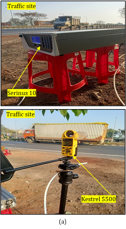
On-site measurements were conducted at a traffic location situated at Kanchdiha (22.382144°N, 87.403331°E) along the National Highway 16 (NH-16) in Kharagpur, West Bengal, India, whereas the background concentration was measured at Jakpur Village (22.375748°N, 87.388626°E) in Kharagpur. NH-16 is commonly known as Chennai-Kolkata Highway which is one of the major and important national highways in India. NH-16 acts as a crucial transportation route connecting major cities along India's eastern coast. The study area lacks any structural or residential development and primarily serves as a thoroughfare for vehicular traffic along the Chennai-Kolkata Highway.

2.2 Sampling technique

The O₃ concentrations were measured using an USEPA-approved method applied instrument (Model: Serinus 10, Make: Acoem, Australia) that utilizes ultraviolet (UV) absorption technology at a wavelength of 254 nm. Data collection took place from 14 – 24^th February, 2023, with observations made from 07:00 to 19:00 each day. To complement the O₃ measurements, a portable weather station (Model: Kestrel 5500, Make: KestrelInstruments, USA), was utilized for the measurement of T, RH, WS and WD. These instruments were positioned at a height of 1.5 meters above the ground surface on the south side of the road, situated 6.7 meters (22 feet) away from the road's edge (Figure 1a) and 14.1 meters away from the pavement road of rural site (Figure 1b). To monitor traffic levels, manual traffic counts were conducted. This involved recording the number of vehicles passing through the study area for a 15-minute duration every hour [18], throughout the entire study duration. Throughout the day, the traffic volume was calculated as vehicles per hour (VPH or veh hr^-1) on a specified segment of this NH-16 within a specific timeframe.

2.3 Multiple linear regression

Regression-based methodologies are commonly used in O₃ prediction studies [38], [39]. Multiple linear regression (MLR) is one of the most widely used methods for modelling O₃ concentrations (dependent or response variable) in dependence of meteorological parameters and different atmospheric pollutants (independent or predictor variables) [37]. Here, in the MLR analysis, the dependent variable that denoted as y_i represents the concentration of O₃. The independent variables that denoted as x_ip denotes regressors T, RH, WS and WD and ∈_i is the error term which explains any unexplained variability in the model. The four regressors denoted as p=1,2,3,4 and n denotes the number of observations. The MLR model can be expressed as follows,

Or,  

Here, i represents the data point, β₀ is the y-intercept, which is the value of 𝑦 when all predictors are zero, β₁,β₂,β₃,β₄ are the coefficients of the model representing the effect of each independent variable on the dependent variable.

3. Results

3.1 Influence of traffic volume on O₃ concentration

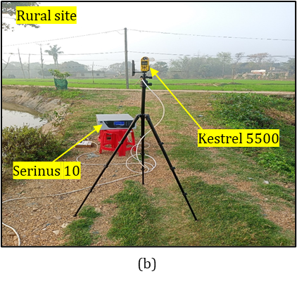
The manually counted vehicle types has been classified into six major categories based on wheels such as motorbikes (2 wheelers), autos (3 wheelers), cars/jeeps/vans (4 wheelers), buses (6 wheelers), light commercial vehicles or LCVs (4 - 6 wheelers), and heavy commercial vehicles or HCVs (6 wheelers or more). These categories represented 32.4%, 1.7%, 25.1%, 2.3%, 13.2%, and 25.3% of the total fleet composition, respectively (Figure 2). Motorbikes and HCVs were the most prevalent vehicle types, whereas autos and buses were comparatively less abundant. From the Figure 2, analysis shows that two wheelers, HCVs and cars were found to be the biggest contributors of emissions of ozone precursors and most frequent vehicle types throughout the day.

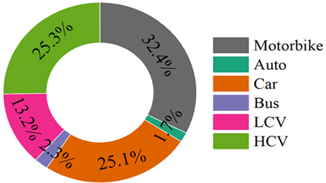
From the Figure 3, it is clear that ozone levels exhibit a strong positive correlation (r = 0.84) with temperature, indicating that as temperature increases, ozone levels tend to increase as well. Conversely, there's a moderate negative correlation (r = -0.53) between ozone and relative humidity, suggesting that as humidity levels increase, ozone levels tend to decrease. Wind speed shows a weak positive correlation (r = 0.075) with ozone, implying a small tendency for ozone levels to increase with higher wind speeds. Wind direction displays a moderate negative correlation (r = -0.39) with ozone, suggesting that a specific wind direction may be linked to lower ozone levels. Moreover, there is a strong negative correlation (r = -0.87) observed between ozone and traffic volume, indicating that higher traffic volume is associated with lower ozone levels.

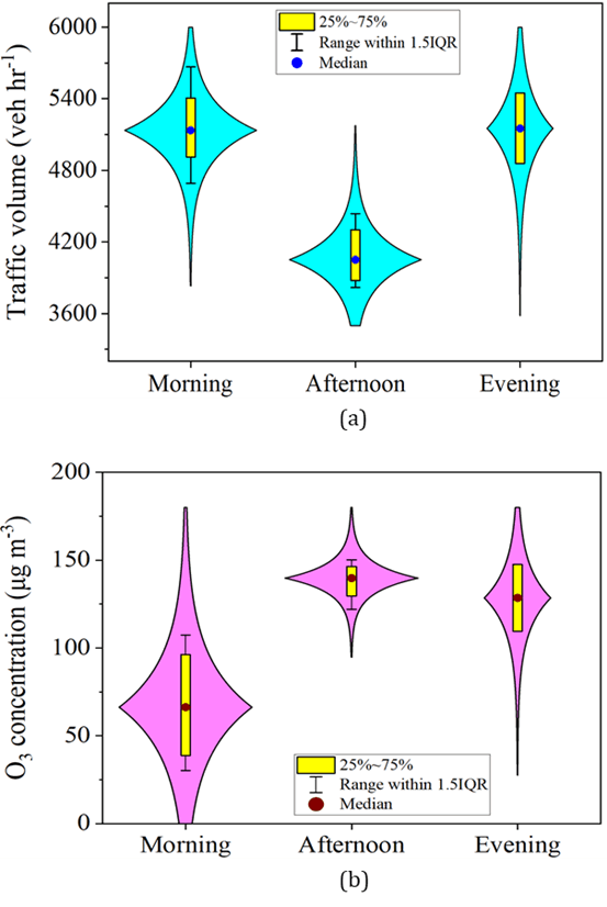
There were fluctuations in traffic volume, with the highest traffic volume occurring in the morning and evening and the lowest traffic volume were observed in the afternoon. Figure 4a and 4b demonstrate a relationship where increased number of vehicles (traffic volume, veh hr^-1), characterized by mixed traffic flow, is associated with decreased O₃ concentration levels during morning and evening hours. An opposite trend was observed during afternoon when low traffic volume is associated with high O₃ concentration levels. This decrement of O₃ concentration levels is primarily attributed to high vehicle volume, which serves as a major contributor to elevated emissions of NO_x, particularly nitric oxide (NO) [19]. These newly emitted NO molecules rapidly react with ozone O₃ molecules [20], [21], leading to the formation of nitrogen dioxide (NO₂) and molecular oxygen (O₂) (NO + O₃ → NO₂ + O₂). As a result, this chemical transformation results in a noticeable decrease in the concentration of GLO [22] during the morning and evening at the traffic site. This phenomenon highlights the significant role of vehicular emissions in influencing GLO chemistry [23], and air quality dynamics in traffic areas [24], [25]. During afternoon, increased O₃ concentration was observed due to decreased traffic volume. This increment of O₃ concentration levels is primarily attributed to the low vehicle volume, so lower emission of fresh NO thus lower destruction of O₃ molecules. Here, high solar insolation during afternoon also comes into the picture of the phenomenon of photochemistry. This photochemistry that influences higher NO₂ to O₃ formation rate during afternoon along with less fresh NO emissions due to low traffic volume is responsible for high O₃ concentration levels at afternoon.

3.2 Influence of meteorology on O₃ concentration

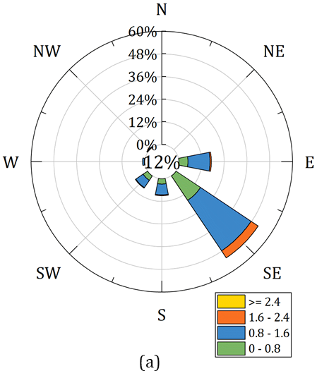
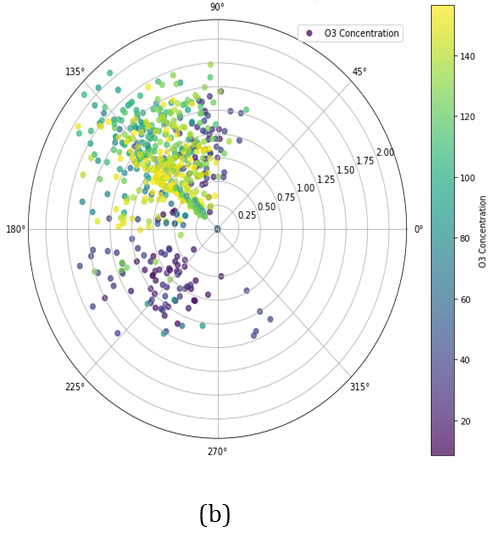
Meteorology showed a substantial impact in O₃ concentration variation for the study sites where temperature strongly positively correlated and relative humidity negatively correlated (Figure 3) and influencing ozone formation and destructions mechanisms. When the wind was blowing from the south-east (SE) to the north-west (NW) (Figure 5a) at a relatively low to moderate speed (0.5 to 1.25 m s^-1), the concentration of O₃ in the air was high (Figure 5b). It was evident that wind speed played a pivotal role in carrying O₃ molecules and their precursors away from the traffic site [26]. The wind was dispersing O₃ molecules and ozone forming precursors (NO_x and VOC) towards the adjacent rural areas located on both the sides of NH-16. When the wind direction shifts, it is likely that other rural areas in close proximity to NH-16 will also be affected by O₃ pollution.

3.3 Prediction and variability of O₃ concentration

The highest concentration of O₃ was recorded more in the traffic site (204.98 μg m^-3) than the rural site (150.64 μg m^-3) during peak hours (afternoon) of O₃ formation but the 12-h (07:00 - 19:00) average O₃ concentration was almost equivalent at both the sites (traffic site 98.45 μg m^-3 and rural site 98.60 μg m^-3). The maximum average 8-h O₃ concentration (09:00 - 17:00) at the traffic site was recorded 117.25 μg m^-3 and at the rural site is 112.56 μg m^-3. Similarly, the maximum 1-hour average (15:30 - 16:30) O₃ concentration at the traffic site is measured 151.32 μg m^-3, and at the rural site is 144.43 μg m^-3.

These measurements revealed that the maximum daily average 8-h (MDA8) GLO concentration exceeded both the NAAQS 2009 and WHO 2021 prescribed standards of 100 μg m^-3 for both sites. This variation can be attributed to the presence of precursors such as NO_x and VOCs originating from traffic emissions. These precursors exhibit rapid changes in line with the photo-stationary state of the NO-NO₂-O₃ chemical system [27]. Additionally, the study observed lower O₃ concentrations during the morning and evening hours, while higher ozone concentrations during the afternoon (Fig. 5). Table 1 provides a comprehensive descriptive analysis of all the essential variables examined in the study. From the table 1, the O₃ concentration ranges from minimum (Min) 30.94 µg m^-3 to maximum (Max) 156.46 µg m^-3, with an average concentration (Avg) of 117.22 µg m^-3 and a standard deviation (SD) of 34.69 for the traffic site. For the Rural site, the O₃ concentration ranges from 41.63 to 150.64 µg m^-3, with an average of 112.56 µg m^-3 and a standard deviation of 29.80. For the Traffic site, the traffic volume (TV) ranges from minimum 3820 to maximum 5668 vehicles per hour, with an average volume of 4551.42 vehicles per hour and a standard deviation of 669.2. For the Rural site, there was no traffic, only pavements were present. Similarly, Min, Max, Avg and SD values are given in Table 1 for the other parameters such as T, RH and WS.

Table 1. Descriptive statistics of study variables for 8-h duration

Study sites	O3 (µg m-3) (Min-Max) Avg ± SD	T (°C)   (Min-Max) Avg ± SD	RH (%)   (Min-Max) Avg ± SD	WS (m s-1) (Min-Max) Avg ± SD	TV (veh hr-1)
Traffic	(30.94-156.46) 117.22 ± 34.69	(23.4-30.33) 28.27 ± 1.46	(22.75-85.25) 57.63 ± 13.52	(0-2.1) 1.05 ± 0.37	(3820-5668) 4551.42 ± 669.2
Rural	(41.63-150.64) 112.56 ± 29.80	(26-36.3) 31.28 ± 2.36	(50.4-84.3) 65.70 ± 8.0	(0-2.5) 0.52 ± 0.54	-

A MLR model is an advanced version of the simple linear regression model designed to analyse data with more than one predictor variable while still predicting a single outcome variable [28], [29]. The analysis revealed the significance of all four chosen regressors T, RH, WS and WD in influencing O₃ concentration. This implied that each of these variables played a role in affecting ozone levels. Specifically, from the Table 2, the temperature had the most substantial impact on O₃ concentration in the traffic area, with a coefficient of 20.95 and a high level of statistical significance at 99%. This suggests that for every 1°C increase in temperature, we observed a corresponding increase in O₃ concentration by 20.95 units. Furthermore, wind speed demonstrated a strong negative influence on O₃ concentration, with a coefficient of -8.85 and a high statistical significance at 99%. This indicates that a one-unit increase in wind speed leads to an 8.85-unit decrease in GLO concentration. In contrast, both wind direction and relative humidity are statistically significant, but their coefficients have comparatively smaller magnitudes in relation to O₃ concentration. These variables still contribute to influencing O₃ levels, though to a lesser extent compared to temperature and wind speed. To evaluate the goodness of fit of this MLR model, AIC, BIC, and the R-squared tests have been conducted. The model yielded values of 4291.42 for AIC, 4312.30 for BIC, and an R-squared of 0.64 suggests that the lower AIC and BIC values, along with a higher R-squared, indicate a strong fit of this model.

From Table 3, it is clear that all the predictor variables have extremely low p-values (0.001 or 0.009), indicating high significance. This emphasizes that all the predictor variables have strong influence on O₃ concentration levels in the rural area. The MLR (R-squared value of 0.67) model explains approximately 67.0% of the variability, suggesting a moderately strong fit. The overall significance test, F-test, indicates a high F-value (241.881) with a low probability (Prob > F = 0.000) indicates that the model is statistically significant. The model suggests that all chosen regressors significantly influence 8-h O₃ concentration at the rural site, with T and RH having the most pronounced effects. Figure 5 portrays a comparative assessment of measured ozone concentrations in relation to their corresponding predicted values for both sites.

Table 2. MLR results of 8-h O₃ concentration for traffic site

O3	Coef.	St.Err.	t-value	p-value	95% confidence	Interval	Sig
T	20.954	0.827	25.35	0	19.329	22.578	***
RH	0.614	0.092	6.70	0	0.434	0.795	***
WS	-8.848	2.808	-3.15	0.002	-14.365	-3.33	***
WD	0.101	0.035	2.88	0.004	0.032	0.171	***
Constant	-514.793	28.906	-17.81	0	-571.592	-457.994	***
Mean dependent var			117.246	SD dependent var			34.658
R-squared			0.641	Number of obs			481
F-test			212.926	Prob > F			0.000
Akaike crit. (AIC)			4291.419	Bayesian crit. (BIC)			4312.299
***p<0.01, **p<0.05, *p<0.1

Table 3. MLR results of 8-h O₃ concentration for rural site

O3	Coef.	St.Err.	t-value	p-value	95% confidence	Interval	Sig
T	-3.308	0.895	-3.69	0	-5.068	-1.549	***
RH	-3.637	0.262	-13.87	0	-4.152	-3.122	***
WS	-5.438	1.664	-3.27	0.001	-8.709	-2.168	***
WD	-0.036	0.014	-2.64	0.009	-0.063	-0.009	***
Constant	465.633	43.974	10.59	0	379.226	522.039	***
Mean dependent var			112.309	SD dependent var			30.010
R-squared			0.670	Number of obs			481
F-test			241.881	Prob > F			0.000
Akaike crit. (AIC)			4112.654	Bayesian crit. (BIC)			4133.534
***p<0.01, **p<0.05, *p<0.1

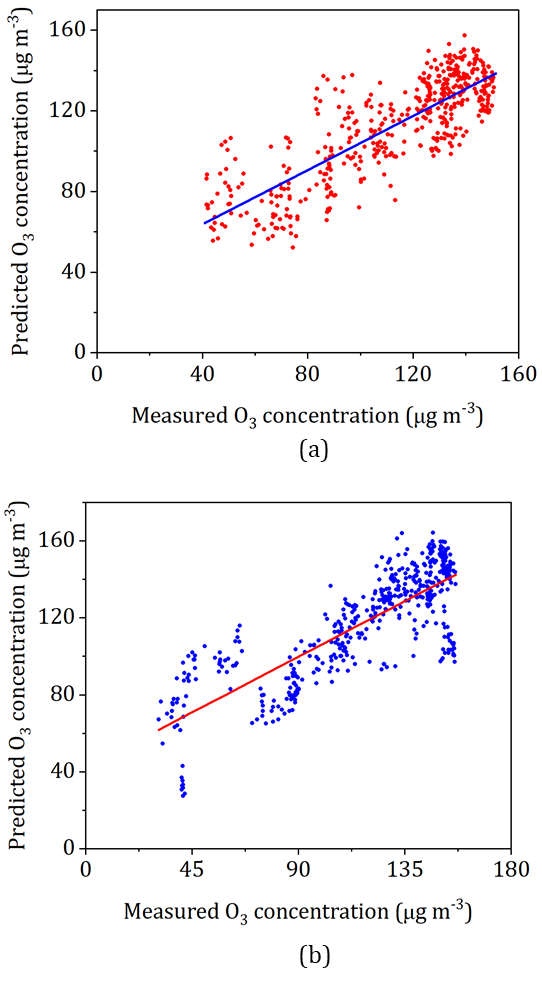
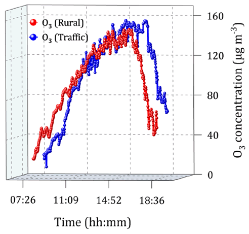
The highest predicted maximum 8-h (09:00 – 17:00) average O₃ concentration for the traffic site was 164.14 μg m^-3 (highest measured 156.46 μg m^-3) and for the rural site was 157.48 μg m^-3 (highest measured 150.64 μg m^-3). Traffic site was more prone to fluctuations in O₃ levels than the rural site because the traffic site was experiencing continuous emissions from running vehicles at all times. O₃ levels were comparatively lower in the morning at the traffic site than at the rural site due to the readily available NO, which reduces O₃ concentration levels. Throughout the fluctuations in concentration levels, O₃ levels were comparatively high during the afternoon, starting a slow decline as the evening approaches. However, in the morning at the rural site, O₃ concentration is comparatively higher than the traffic site due to the absence of NO, resulting in less reduction of O₃ concentration levels. O₃ levels at the rural site show a gradual increasing trend throughout the day, reaching peak levels during the afternoon (though comparatively lower in concentration than at the traffic site). As evening approaches, there is a rapid, steady fall in O₃ concentration levels due to non-availability of precursors in ozone formation. Depending on the above-mentioned phenomena, O₃ concentration profile for both traffic site and rural site is shown in Figure 6. This ozone profile is clearly showing the diurnal variability of O₃ concentration.

The dynamics of ozone are complicatedly influenced by various gases present in the traffic environment from the direct emissions or formed from primary emissions (Figure 7). Increased traffic leads to increased emissions of O₃ precursor gases, such as VOCs, particularly in the morning and evening. However, despite the elevated levels of VOCs, the reduced sunlight intensity during these periods doesn't proportionally increase ozone formation [40]. In the presence of adequate NO_x, non-methane hydrocarbons (NMHCs) play a significant role in enhanced formation of O₃ molecules [41].  In the Figure 7, the cyclic process of O3 formation and discussion, hydroxyl radicals (^.OH), generated from the interaction of water vapor with O₃, and then undergoes subsequent reactions to form hydroperoxyl radicals (HO^.₂), thus contribute to a decrease in O₃ levels. However, under adequate sunlight, these radicals facilitate O₃ formation [42], [43]. Additionally, in the presence of ^.OH, carbon monoxide (CO) contributes to ozone formation [21]. Figure 7 displays that O₃ molecule in the troposphere under solar radiation (λ < 330 nm) breaks into atomic oxygen O(³P) and exited oxygen O(¹D). This atomic oxygen further reacts with oxygen molecule (O₂) with the presence of third body (M = O₂, N₂) and forms O₃ molecule whereas O(¹D) joins the cyclic process of RO_x cycle, NO_x cycle with presence of VOCs and CO, it leads to the formation and destruction of O₃ molecules.

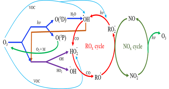
In the traffic environment, this cyclic process of O₃ formation is higher during mid-day with high insolation associated with low NO molecules availability and destruction is high during morning and evening due to low insolation associated with high availability of NO molecules. Therefore, the traffic environment is strongly dominated by the NO_x cycle. But in case of the rural site, it is mostly dominated by RO_x cycle where chemical reactions, pollutants accumulation, atmospheric stability, local wind circulation patterns, and biogenic emissions may be the reasons of high O₃ concentration levels.

4. Discussions

The study provides insightful observations regarding the complex relationship between traffic volume, meteorological conditions, and ozone concentration at both traffic and rural sites. Notably, it explains the dynamic connections of various factors influencing O₃ levels throughout the day. One significant finding is the pronounced negative correlation (-0.87) between traffic volume and O₃ concentration, particularly during peak traffic hours. This correlation highlights the substantial impact of vehicular emissions, especially NO_x, on O₃ dynamics. The observed decrease in O₃ concentration during high traffic periods is attributed to the rapid reaction between newly emitted NO molecules and O₃, forming nitrogen dioxide (NO₂) and molecular oxygen (O₂). Conversely, during periods of low traffic volume, O₃ concentration tends to increase due to reduce NO emissions and enhanced photochemistry of NO₂ to O₃ formation under high solar insolation. Meteorological factors, particularly temperature and wind speed, also play pivotal roles in modulating O₃ levels. Temperature exhibited a strong positive correlation with O₃ concentration, indicating its role in promoting O₃ formation. Wind speed, on the other hand, demonstrated a negative influence on O₃ concentration, as it aids in dispersing O₃ molecules and their precursors away from the traffic site. The MLR analysis explained the significance of T, RH, WS and WD in predicting O₃ concentration. These findings capture the complex mechanisms of meteorological variables in shaping O₃ dynamics. Furthermore, the study explored the discrepancy in O₃ concentration between traffic and rural sites where traffic site was exhibiting higher variability and fluctuations due to continuous vehicular emissions. This discrepancy underscores the need for targeted interventions to mitigate vehicular emissions and alleviate O₃ pollution in urban traffic areas. Overall, findings contribute valuable insights for policymakers and urban planners in planning effective strategies to mitigate O₃ pollution and enhance air quality in traffic environments.

5. Conclusions

The O₃ pollution levels over an 8-h period has been found to exceed the prescribed standards for both NAAQS 2009 and WHO 2021 along NH-16 in Kharagpur, India. Interestingly, there is a significant negative correlation (r = -0.87) between traffic volume and O₃ concentration, indicating that high traffic volume is associated with lower O₃ levels. Temperature shows a positive correlation, while relative humidity is negatively correlated with O₃ concentration. Moderate wind speed from south-east (SE) direction shows elevated O₃ levels at the study site and carrying O₃ molecules and their precursors away from the traffic area and contributing high O₃ levels in the nearby rural areas. When wind direction changes, it is likely that nearby rural areas along NH-16 will also be affected by these pollutants. The most suitable model for predicting O₃ concentration is MLR, as supported by the R-squared, AIC, and BIC analyses. This model successfully predicts O₃ pollution levels along NH-16 in Kharagpur, with the highest predicted concentration at 164.14 μg m^-3 (highest measured 156.46 μg m^-3). In light of these findings, urgent action is required to establish a comprehensive screening process for assessing O₃ pollution levels along all national highways in India. It is extremely necessary to conduct further investigations on other highways and formulate a new policy which will aim to effectively address and mitigate GLO pollution levels along the national highways in India.

References

[1] N. Qian, 'Bottled Water or Tap Water? A Comparative Study of Drinking Water Choices on University Campu[1] Horstman, "Pulmonary function and symptom responses after 6.6-hour exposure to 0.12 ppm ozone with moderate exercise," JAPCA, vol. 38, no. 1, pp. 28-35, 1988. View Article
[2] P. J. Crutzen, "The role of NO and NO2 in the chemistry of the troposphere and stratosphere," Annu. Rev. Earth Planet. Sci., vol. 7, no. 1, pp. 443-472, 1979. View Article
[3] B. Sadeghi, M. Ghahremanloo, S. Mousavinezhad, Y. Lops, A. Pouyaei, and Y. Choi, "Contributions of meteorology to ozone variations: Application of deep learning and the Kolmogorov-Zurbenko filter," Environ. Pollut., vol. 310, pp. 119863, 2022. View Article
[4] A. Calle-Martínez, R. Ruiz-Páez, L. Gómez-González, A. Egea-Ferrer, J. A. López-Bueno, J. Díaz, C. Asensio, M. A. Navas, and C. Linares, "Short-term effects of tropospheric ozone and other environmental factors on emergency admissions due to pregnancy complications: A time-series analysis in the Madrid Region," Environ. Res., vol. 231, no. Pt 2, p. 116206, 2023. View Article
[5] P. Cheng, C. Liu, B. Tu, X. Zhang, F. Chen, J. Xu, D. Qian, X. Wang, and W. Zhou, "Short-Term effects of ambient ozone on the risk of conjunctivitis outpatient visits: a time-series analysis in Pudong New Area, Shanghai," Int. J. Environ. Health Res., vol. 33, no. 4, pp. 348-357, 2023. View Article
[6] X. Wang, J. Cai, X. Liu, B. Wang, L. Yan, R. Liu, Y. Nie, Y. Wang, X. Zhang, and X. Zhang, "Impact of PM2.5 and ozone on incidence of influenza in Shijiazhuang, China: a time-series study," Environ. Sci. Pollut. Res. Int., vol. 30, no. 4, pp. 10426-10443, 2023. View Article
[7] C. Chen, T. Li, Q. Sun, W. Shi, M. Z. He, J. Wang, J. Liu, M. Zhang, Q. Jiang, M. Wang, and X. Shi, "Short-term exposure to ozone and cause-specific mortality risks and thresholds in China: Evidence from nationally representative data, 2013-2018," Environ. Int., vol. 171, p. 107666, 2023. View Article
[8] A. R. Soares and C. Silva, "Review of Ground-Level Ozone Impact in Respiratory Health Deterioration for the Past Two Decades," Atmosphere, vol. 13, no. 3, p. 434, 2022. View Article
[9] B. E. Tilton, "Health effects of tropospheric ozone," Environ. Sci. Technol., vol. 23, no. 3, pp. 257-263, 1989. View Article
[10] M. S. Reddy and C. Venkataraman, "Inventory of aerosol and sulphur dioxide emissions from India: I-Fossil fuel combustion," Atmos. Environ., vol. 36, no. 4, pp. 677-697, 2002. View Article
[11] A. Srivastava, B. Sengupta, and S. A. Dutta, "Source apportionment of ambient VOCs in Delhi City," Sci. Total Environ., vol. 343, no. 1-3, pp. 207-220, 2005. View Article
[12] L. Camalier, W. Cox, and P. Dolwick, "The effects of meteorology on ozone in urban areas and their use in assessing ozone trends," Atmos. Environ., vol. 41, no. 33, pp. 7127-7137, 2007. View Article
[13] L. Tong, H. Zhang, J. Yu, M. He, N. Xu, J. Zhang, F. Qian, J. Feng, and H. Xiao, "Characteristics of surface ozone and nitrogen oxides at urban, suburban and rural sites in Ningbo, China," Atmos. Res., vol. 187, pp. 57-68, 2017. View Article
[14] S. Tyagi, S. Tiwari, A. Mishra, P. K. Hopke, S. D. Attri, A. K. Srivastava, and D. S. Bisht, "Spatial variability of concentrations of gaseous pollutants across the National Capital Region of Delhi, India," Atmos. Pollut. Res., vol. 7, no. 5, pp. 808-816, 2016. View Article
[15] B. S. K. Reddy, K. R. Kumar, G. Balakrishnaiah, K. R. Gopal, R.R. Reddy, V. Sivakumar, A.P. Lingaswamy, S. Md. Arafath, K. Umadevi1, S. P. Kumari, Y. N. Ahammed, and S. Lal, "Analysis of Diurnal and Seasonal Behavior of Surface Ozone and Its Precursors (NOx) at a Semi-Arid Rural Site in Southern India," Aerosol Air Qual. Res., vol. 12, no. 6, pp. 1081-1094, 2012. View Article
[16] B. S. Nelson, G. J. Stewart, W. S. Drysdale, M. J. Newland, A. R. Vaughan, R. E. Dunmore, P. M. Edwards, A. C. Lewis, J. F. Hamilton, W. J. A. C. Nicholas Hewitt, L. R. Crilley, M. S. Alam, Ü. A. Şahin, D. C. S. Beddows, W. J. Bloss, E. Slater, L. K. Whalley, D. E. Heard, J. M. Cash, B. Langford, E. Nemitz, R. Sommariva, S. Cox, Shivani, R. Gadi, B. R. Gurjar, J. R. Hopkins, A. R. Rickard, and J. D. Lee, "In situ ozone production is highly sensitive to volatile organic compounds in Delhi, India," Atmospheric Chemistry and Physics, vol. 21, no. 17, pp. 13609-13630, 2021. View Article
[17] A. K. Paschalidou, P. A. Kassomenos, and A. Bartzokas, "A comparative study on various statistical techniques predicting ozone concentrations: implications to environmental management," Environ. Monit. Assess., vol. 148, no. 1-4, pp. 277-289, 2009. View Article
[18] N. Singh, N. Chauhan, N. Pande, and N. M. Prasad, "Traffic volume study and congestion solutions," IJEAST, vol. 6, no. 7, pp. 307-321, 2021. View Article
[19] A. K. Nagpure, B. R. Gurjar, and N. Sahni, "Pollutant emissions from road vehicles in megacity Kolkata, India: past and present trends," Indian Journal of Air Pollution Control, vol. X, no. 2, pp. 18-30, 2010.
[20] K. Glaser, "Vertical profiles of O3, NO2, NOx, VOC, and meteorological parameters during the Berlin Ozone Experiment (BERLIOZ) campaign," J. Geophys. Res., vol. 108, no. D4, p. 8253, 2003. View Article
[21] M. Trainer, D. D. Parrish, M. P. Buhr, R. B. Norton, F. C. Fehsenfeld, K. G. Anlauf, J. W. Bottenheim, Y. Z. Tang, H. A. Wiebe, J. M. Roberts, R. L. Tanner, L. Newman, V. C. Bowersox, J. F. Meagher, K. J. Olszyna, M. O. Rodgers, T. Wang, H. Berresheim, K. L. Demerjian, and U. K. Roychowdhury, "Correlation of ozone with NOy in photochemically aged air," J. Geophys. Res., vol. 98, no. D2, pp. 2917-2925, 1993. View Article
[22] S. Munir, H. Chen, and K. Ropkins, "Modelling the impact of road traffic on ground level ozone concentration using a quantile regression approach," Atmos. Environ., vol. 60, pp. 283-291, 2012. View Article
[23] S. Munir, H. Chen, and K. Ropkins, "Characterising the temporal variations of ground-level ozone and its relationship with traffic-related air pollutants in the United Kingdom: a quantile regression approach," Int. J. SDP, vol. 9, no. 1, pp. 29-41, 2014. View Article
[24] M. Schmidt and R. P. Schäfer, "An integrated simulation system for traffic induced air pollution," Environmental Modelling & Software, vol. 13, no. 3-4, pp. 295-303, 1998. View Article
[25] R. Garaga, S. K. Sahu, and S. H. Kota, "A review of air quality modeling studies in india: local and regional scale," Curr. Pollution Rep., vol. 4, no. 2, pp. 59-73, 2018. View Article
[26] K. Li, L. Chen, F. Ying, S. J. White, C. Jang, X. Wu, X. Gao, S. Hong, J. Shen, M. Azzic, K. Cena, "Meteorological and chemical impacts on ozone formation: A case study in Hangzhou, China," Atmos. Res., vol. 196, no. 1, pp. 40-52, 2017. View Article
[27] I. Trebs, O. L. Mayol-Bracero, T. Pauliquevis, U. K., R. Sander, L. Ganzeveld, F. X. Meixner, J. Kesselmeier, P. Artaxo, M. O. Andreae, "Impact of the Manaus urban plume on trace gas mixing ratios near the surface in the Amazon Basin: Implications for the NO-NO2 -O3 photostationary state and peroxy radical levels," J. Geophys. Res., vol. 117, no. D5, 2012. View Article
[28] L. E. Eberly, "Multiple linear regression," in Methods Mol. Biol., W. T. Ambrosius, Ed. Totowa New Jersey: Humana Press, vol. 404, pp. 165-187, 2007. View Article
[29] M. Arsić, I. Mihajlović, D. Nikolić, Ž. Živković, and M. Panić, "Prediction of ozone concentration in ambient air using multilinear regression and the artificial neural networks methods," Ozone: Science & Engineering, vol. 42, no. 1, pp. 79-88, 2020. View Article
[30] D. J. Ball, "A history of secondary pollutant measurements in the London region 1971-1986," Science of The Total Environment, vol. 59, pp. 181-206, 1987. View Article
[31] F. Geng, X. Tie, J. Xu, G. Zhou, L. Peng, W. Gao, X. Tang, C. Zhao, "Characterizations of ozone, NOx, and VOCs measured in Shanghai, China," Atmospheric Environment, vol. 42(29), pp. 6873-6883, 2008. View Article
[32] A. Singh, S. Gangopadhyay, P. K. Nanda, S. Bhattacharya, C. Sharma, C. Bhan, "Trends of greenhouse gas emissions from the road transport sector in India," The Science of the Total Environment, vol. 390(1), pp. 124-131, 2008. View Article
[33] S. M. T, and H. J. Bhasin, "Empirical Study of Consumption Pattern of Petrol and Diesel According to Regions in India," Social Science Journal, vol. 13. no. 3, pp. 3445-3456, 2023.
[34] M. R. Nouni, P. Jha, R. Sarkhel, C. Banerjee, A. K. Tripathi, J. Manna, "Alternative fuels for decarbonisation of road transport sector in India: Options, present status, opportunities, and challenges," Fuel, vol. 305, 121583, 2021. View Article
[35] M. Naja, and S. Lal, "Changes in surface ozone amount and its diurnal and seasonal patterns, from 1954-55 to 1991-93, measured at Ahmedabad (23 N), India," Geophysical Research Letters, vol. 23(1), pp. 81-84, 1996. View Article
[36] N. Ojha, M. Naja, K. P. Singh, T. Sarangi, R. Kumar, S. Lal, M. G. Lawrence, T. M. Butler, and H. C. Chandola, "Variabilities in ozone at a semi‐urban site in the Indo‐Gangetic Plain region: Association with the meteorology and regional processes," Journal of Geophysical Research, vol. 117(D20301), 2012. View Article
[37] N. R. Awang, N. A. Ramli, A. S. Yahaya, and M. Elbayoumi, "Multivariate methods to predict ground level ozone during daytime, nighttime, and critical conversion time in urban areas", Atmospheric Pollution Research, vol. 6(5), pp. 726-734, 2015. View Article
[38] S. Bekesiene, I. Meidute-Kavaliauskiene, and V. Vasiliauskiene, "Accurate prediction of concentration changes in ozone as an air pollutant by multiple linear regression and artificial neural networks," Mathematics, vol. 9(4), pp. 356, 2021. View Article
[39] W. Zhao, S. Fan, H. Guo, B. Gao, J. Sun, and L. Chen, "Assessing the impact of local meteorological variables on surface ozone in Hong Kong during 2000-2015 using quantile and multiple line regression models," Atmospheric Environment, vol. 144, pp. 182-193, 2016. View Article
[40] T. T. Hien, D. H. Huy, P. A. Dominutti, N. D. Thien Chi, J. R. Hopkins, M. Shaw, G. Forster, G. Mills, H. A. Le, and D. Oram, "Comprehensive volatile organic compound measurements and their implications for ground-level ozone formation in the two main urban areas of Vietnam," Atmospheric Environment, vol. 269, 118872, 2022. View Article
[41] C. Jia, X. Mao, T. Huang, X. Liang, Y. Wang, Y. Shen, W. Jiang, H. Wang, Z. Bai, M. Ma, Z. Yu, J. Ma, and H. Gao, "Non-methane hydrocarbons (NMHCs) and their contribution to ozone formation potential in a petrochemical industrialized city, Northwest China," Atmospheric Research, vol. 169, pp. 225-236, 2016. View Article
[42] M. Lily, S. Hynniewta, B. Muthiah, W. Wang, A. K. Chandra, and F. Liu, "Quantum chemical insights into the atmospheric reactions of CH2FCH2OH with OH radical, fate of CH2FC•HOH radical and ozone formation potential," Atmospheric Environment, vol. 249, 118247, 2021. View Article
[43] Z. Tan, K. Lu, A. Hofzumahaus, H. Fuchs, B. Bohn, F. Holland, Y. Liu, F. Rohrer, M. Shao, K. Sun, Y. Wu, L. Zeng, Y. Zhang, Q. Zou, A. Kiendler-Scharr, A. Wahner, and Y. Zhang, "Experimental budgets of OH, HO2, and RO2 radicals and implications for ozone formation in the Pearl River Delta in China 2014," Atmospheric Chemistry and Physics, vol. 19(10), pp. 7129-7150, 2019.
[44] Anshika, R. K. Kunchala, R. Attada, R. K. Vellore, V. K. Soni, M. Mohan, and N. Chilukoti, "On the understanding of surface ozone variability, its precursors and their associations with atmospheric conditions over the Delhi region," Atmospheric Research, vol. 258, 105653, 2021. View Article