International Journal of Environmental Pollution and Remediation (IJEPR)

ISSN: 1929-2732

1. Introduction

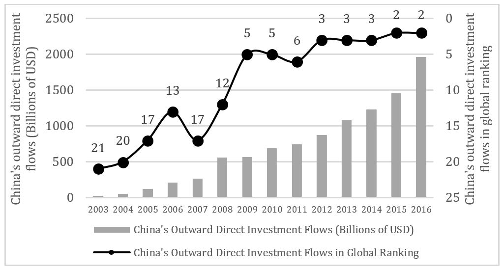
Since the implementation of “Going Out” strategy after WTO accession in the 2000s, China’s outward foreign direct investment (OFDI) has skyrocketed, especially when China has ushered into a “New Normal” era, as accompanied with a series of global policies and economic strategies (e.g., the proposal of the One Belt & One Road initiative (BRI) and establishment of the Asian Infrastructure Investment Bank (AIIB) unveiled in the 2010s after the world economic and financial crisis). According to the Statistical Bulletin of China’s Outward Foreign Direct Investment (Figure 1), China’s OFDI flows first exceeded the amount of inward foreign direct investment (IFDI) in 2015. Moreover, newly increased OFDI by Chinese domestic investors rapidly rose to $1456.7 billion in 2015 from only $28.5 billion in 2003, ranking second worldwide, making it a true investment country.

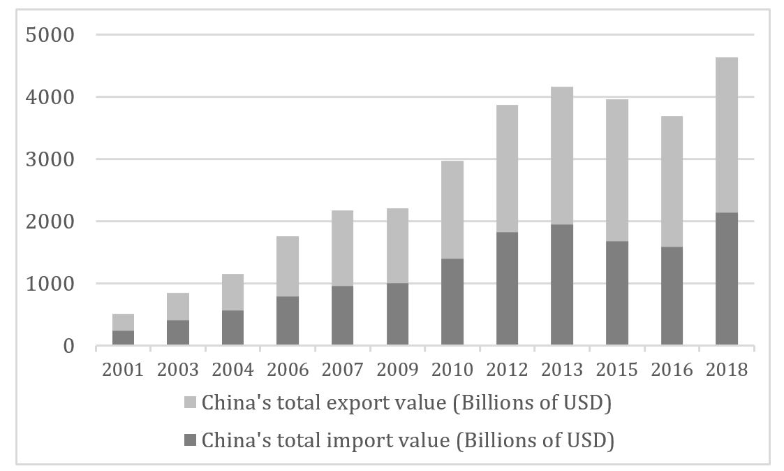
Moreover, as one of the critical sectors of economic growth, foreign trade in China has been overall undergoing steady growth, especially since its WTO accession in 2001. According to the China General Administration of Customs (Figure 2), China’s total trade value monotonously increases until 2009 affected by the world economic crisis and weak global demand. Subsequently, as the world’s largest trading nation since 2013 and largest bilateral trading partner for most countries, China’s total trade value peaked at $4301.53 billion in 2014, when China has ushered into the“New Normal” era with ongoing industrial upgrading.

2. Literature Reviews

Currently, existing literature on the relationship of investment facilitation & trade liberalization and environment suggests a potentially high level of interaction. To be specific, Grossman and Kruger [1] first decomposed the impact mechanism of foreign direct investment (FDI) on the environment into three channels: scale effect, composition effect, and technique effect, which exert different or even reversed impacts on the environment respectively. Inspired by the mentioned study, Feng [2] determined the relationship between inflows of FDI and local air pollution in China, suggesting that FDI can facilitate a developing country’s environment when the multinationals crowd out inefficient local firms, change the industrial composition, advance technology and boost productivity & energy efficiency. Likewise, Eskeland and Harrison [3] identified little support for the pollution haven hypothesis when the U.S. invests in four countries (Cote d'Ivoire, Mexico, Morocco, and Venezuela). Also, they reported that foreign plants are significantly more energy-efficient and use cleaner types of energy than domestic-owned plants. However, at a larger scale, Grimes et al. [4] analyzed 66 less developed countries, suggesting that foreign investment is more concentrated in those industries that require more energy and positively linked with local carbon dioxide (CO₂) emissions. Besides, transnational corporations may relocate highly polluting industries to countries with fewer environmental controls. Furthermore, Hoffman et al. [5] performed the Granger causality test to delve into the relationships between FDI and CO₂ emissions in 112 countries at different income levels. It was reported that FDI inflows in middle-income countries will promote CO₂ emissions, whereas no such significant relationship was identified in high-income countries. In low-income countries, however, CO₂ emissions can even hinder the entry of FDI.

Given environmental pollution embodied in international trade, Shui and Harriss [6] verified that 7%-14% of China’s CO₂ emissions are caused by its exports to the United States. Inversely, Wyckoff and Roop [7] calculated the embodied carbon emissions in manufactured goods imported by the OECD countries, taking up nearly 13% of its overall emissions. At a larger scale, Peters and Hertwich [8] exploited the input-output data of 2001 to delve into the embodied carbon emissions in international trade in 87 countries. It was reported that carbon emissions embodied in international trade took up 1/4 of the world’s total emissions, with China’s exports and imports carbon emissions respectively accounting for 24% and 7% of its domestic carbon emissions.

Moreover, concerning the role of institutional factors related to China in cross-border investment and trade. Kolstad and Wiig [9] reported that institutional quality of host country exhibits a negative correlation with China’s OFDI, which is attracted to large markets (OECD countries), and countries with a combination of considerable natural resources and poor institutions (non-OECD countries). Likewise, Cheung and Qian [10] utilized China’s OFDI data to Africa, indicating that corruption and legal defects in the region have positive impacts on China’s OFDI. Generally, Habib and Zubawicki [11] proposed that global FDI is not likely to introduce under a severe level of corruption in the host country, while Aleksynska and Havrylchyk [12] suggested that especially for the southern countries, the greater institutional distance will hinder the FDI inflow.

Thus, since the global climate change with increasing greenhouse gas (GHG) emissions is becoming a contentious issue worldwide, and when China’s economy is developing in a broader and more advanced manner, with the emerging process of growing overseas investment and transitions in industrial and trade structure. China’s OFDI and foreign trade will likely pose global environmental issues other than economic benefits, as it is becoming the second-largest investor (inflows) and the largest industrializing & trading nation globally. Thus, in this emerging field rarely discussed by existing studies, the present study will first aim to demonstrate the link of impacts exerted by China (e.g., its overseas investment and foreign trade) and economic and institutional distances with China on CO₂ emissions per capita of 146 countries & regions (2003 to 2016), which is achieved based on the fixed effects-two stage least squares (FE-2SLS) with instrumental variables controlling over endogeneity. Next, it is noteworthy that the threshold regression model with fixed effects is adopted to capture how those China’s overseas economic activities will impact global air pollution, at various phases of economic or institutional distance by taking it as structural breaks or threshold regimes.

3. Threshold Regression Model

The threshold model was introduced by Tong (1978), Tong and Lim (1980), which are overall employed in discrete time series that exhibit piece-wise linearity [13]. Subsequently, the threshold models and other nonlinear time series models have led to the development and sometimes the re-discovery of numerous data analytic techniques [14]. Given the definition of the threshold model, coefficients in the model are inconstant and can be altered by the endogenously determined threshold variables. Furthermore, it allows to split the sample into different regimes, so it is not required to enter dummy variables based on unknown structural breaks [15].

A single threshold regression model with fixed effects is written in Eq. 1

Where i and t indicate area and time effect respectively, I (・) represents an indicator function, it is equal to 1 (there exists a single-threshold effect) or 0 (there exists a linear effect). q_it denotes the threshold variable which refers to the economic or institutional distances in the present study. γ represents the threshold value that divides the equation into two regimes with different threshold coefficients of β₁ and β₂. Besides, X_it denotes the core explanatory variable that respectively refers to China’s overseas investment or imports respectively, and y_it represents the explained variable refers to CO₂ emissions per capita of 146 countries & regions. Lastly, X'_it in the present study is a set of control variables representing the rest of variables other than threshold variable that bring a linear relationship on explained variable with coefficient θ’, while μ_i represents the individual effect and ε_it indicates the disturbance term. Moreover, individual fixed effect (µ_i) will be eliminated via fixed effect transformation by deducting its own average value in the present study.

Commonly, the estimated threshold value (γ(_)) can be derived by minimizing the residual sum of squared errors , and once the threshold value is obtained, the corresponding parameter estimates of threshold (β(_)) will be given by the ordinary least squares [16].

Here, when the test is performed on the significance of threshold effect at a relevant confidence level, whether there exists a threshold effect is verified, which satisfies the purpose of verifying whether the coefficients are identical in the respective regime, i.e., the null hypothesis (H₀: β₁=β₂) against the alternative hypothesis (H₁: β₁≠β₂). Accordingly, the null hypothesis (of linearity) can be rejected, a single threshold effect nonlinear regression will take place (with two threshold regimes). Besides, the F statistic under the null hypothesis is defined in Eq. 2 as

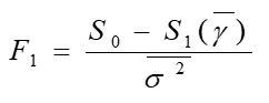
Where the S₁ and S₀ respectively denote the residual sum of squared errors with and without threshold effect respectively,  indicates the variance of the residual. Given the null hypothesis of H₀, the threshold value is not identified, and F₁ exhibits a nonstandard asymptotic distribution. Accordingly, Hansen in 1999 developed a repetitive bootstrap approach on the critical values of the F statistic, as an attempt to make the statistic asymptotically distributed and verify the significance of the threshold effect by determining the asymptotic p-values [17]. In the present study, it will run 1000 bootstraps by Stata 15.

4. Data and Variables

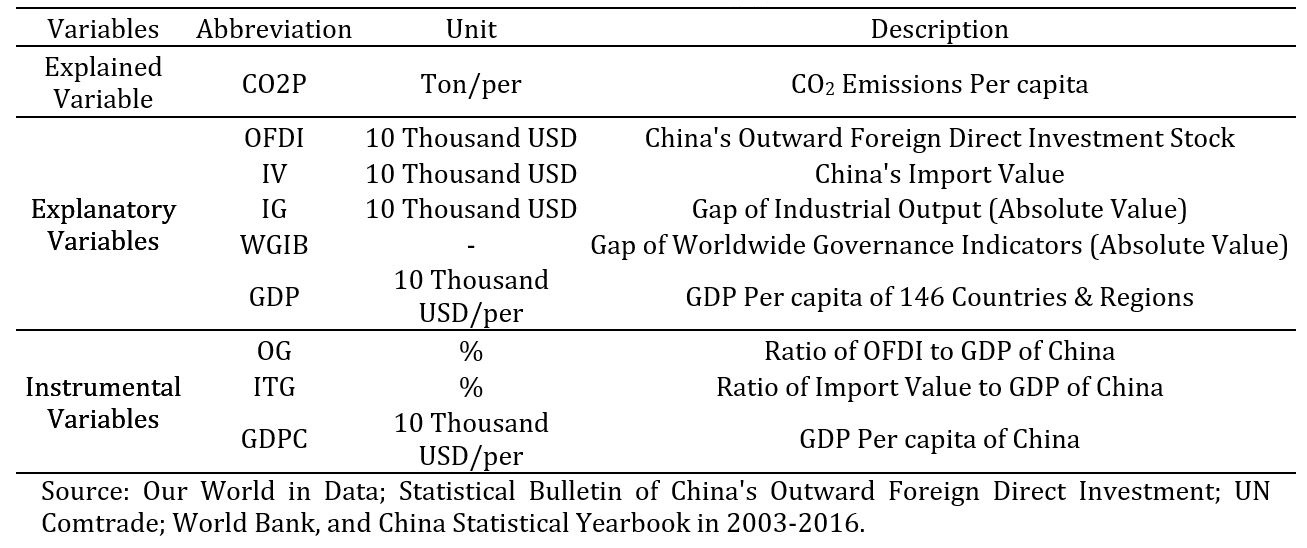
Given the availability and representativeness of data, the variables applied in the present study packing in a panel set of 146 countries & regions (2003 to 2016) are listed in Table 1. Here, “CO₂ Emissions Per capita” (ton/per, CO2P) of 146 countries & regions are represented as explained variable. Besides, “China's Outward Foreign Direct Investment Stock” (10 Thousand USD, OFDI) and “China's Import Value” (10 Thousand USD, IV) are set as core explanatory variables respectively. “Gap of Industrial Output” (10 Thousand USD, IG) and “Gap of Worldwide Governance Indicators” (WGIB) in absolute value are treated as threshold variable respectively to verify the relevant threshold effect in threshold model, and “GDP (Nominal) Per capita” (10 Thousand USD/per, GDP) of 146 Countries & Regions is regarded as the control variable. As a supplement, “Ratio of OFDI to GDP” (%, OG), “Ratio of Import Value to GDP” (%, ITG) and “GDP Per capita” (10 Thousand USD/per, GDPC) of China are adopted as instrumental variables conducted in fixed effects-two stage least squares. In addition, the present study will transform the variables into logarithms to reduce the fluctuation of the model without changing the assessment trend.

Table 1. Definitions of applied variables.

5. Regression Analysis and Estimates

Based on the applied panel data of 146 countries & regions in 2003-2016, this paper will conduct the fixed effects-two stage least squares with instrumental variables controlling the endogeneity, and threshold regression model with fixed effects, respectively, to check the estimates mutually and capture how China’s overseas economic activities will impact global air pollution, at various phases of economic or institutional distance.

5. 1. Fixed Effects-Two Stage Least Squares

The endogeneity problem arises when explanatory variables and the error term are correlated, or omitted variable is confounding both independent and dependent variables [18]. Accordingly, fixed effects-two stage least squares will be utilized in the present study by employing exogenous instrumental variables to perform the endogenous bias correction, based on various of corresponding tests and results in Table 2.

Table 2. Fixed effects-two stage least squares model estimate.

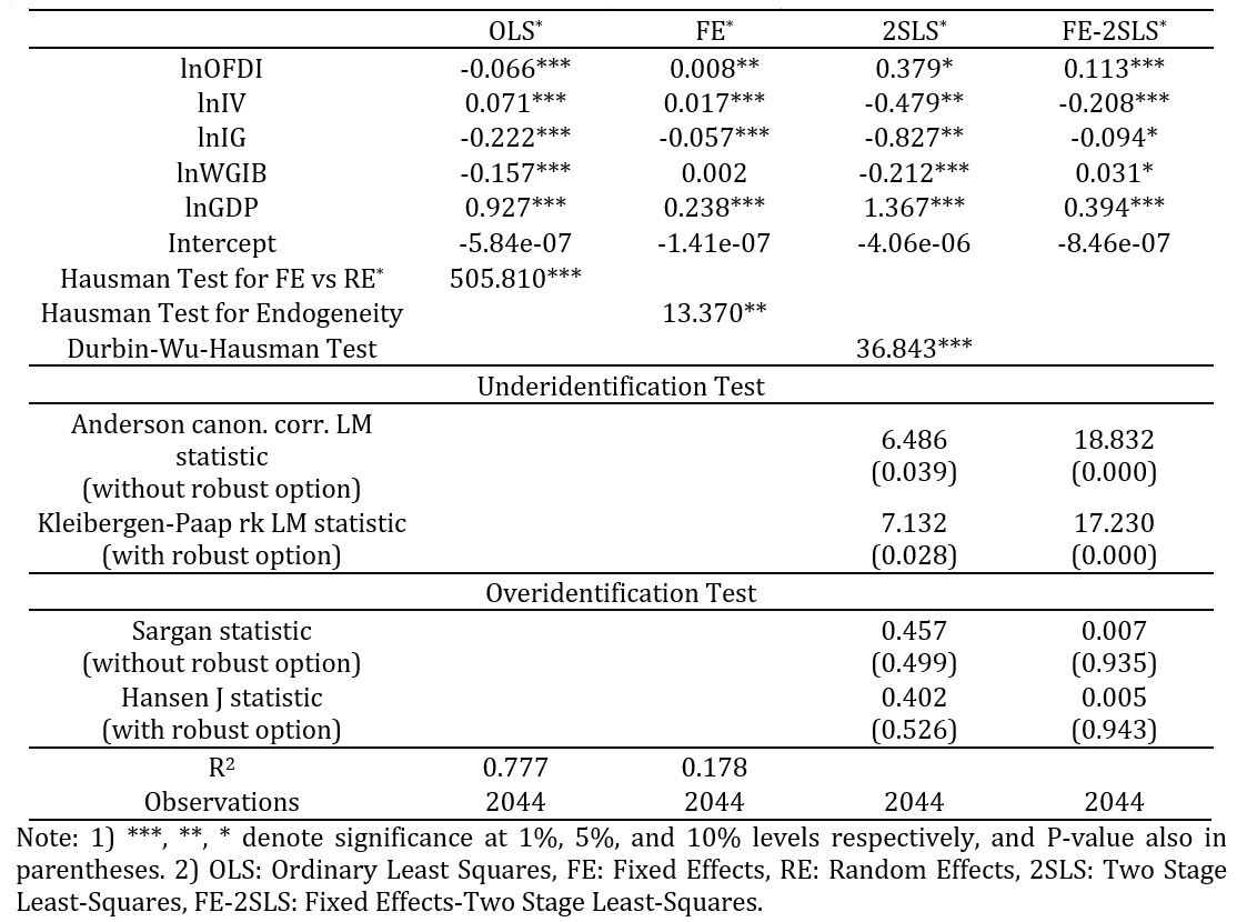
To be specific, when OG (Ratio of OFDI to GDP), ITG (Ratio of Import Value to GDP), and GDPC (GDP Per capita) of China are taken as instrumental variables for OFDI and IV considering endogenous explanatory variables, the null hypothesis of Hausman test for endogeneity (H₀: Explanatory variables are exogenous) and Durbin-Wu-Hausman (DWH) test (H₀: Endogenous regressors are in fact exogenous) are both rejected in a statistically significant manner, demonstrating that OFDI and IV are indeed endogenous explanatory variables in the present study. Subsequently, the implementation of the instrumental variables will be verified by the underidentification test on the correlation between instrumental variables and endogenous explanatory variable (H₀: Instrumental variables are not correlated with endogenous explanatory variable) and by the overidentification test on the exogeneity of instrumental variables (H₀: Instrumental variables are not correlated with disturbance term), which are supported to be valid.

Accordingly, how the assessed results of the FE-2SLS controlling endogenous bias differ from the results of the FE in Table 2 suggest that the OFDI distinctly exhibits a higher positive coefficient (0.113) significantly. It is therefore revealed that instrumental variables of the OG, ITG and GDPC, representing China’s development of overseas economic cooperation, tend to positively impact the global level of CO₂ emission. In contrast, IV in FE-2SLS turns into opposite and negative coefficient (-0.208) significantly compared with the result in FE, which can be interpreted as a CO₂ mitigation effect concealed in China’s global imports when China’s economy is transforming to a more open and mature market.

5. 2. Threshold Regression Model with Fixed Effects

On that basis, the threshold regression model with fixed effects will be simulated to capture how China’s OFDI and imports will impact air pollution of 146 countries & regions, under every phase of economic or institutional distance treated as threshold regimes. Simultaneously, given the lagged effects of overseas investment and international trade, along with the correction for the endogenous problem on some level, assessment of the threshold regression model in the present study will apply one-year lagged OFDI and IV as core explanatory variables.

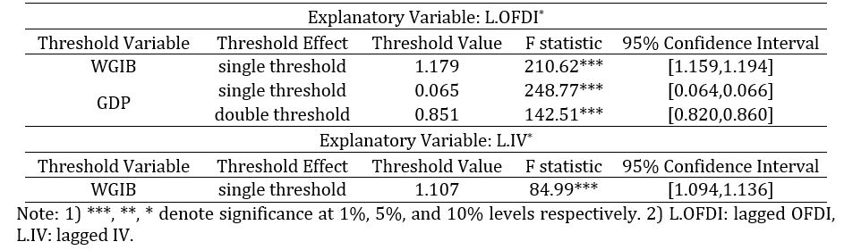
First, the threshold effect test will be performed in Table 3, separated in the relationship of L.OFDI (One year lag OFDI) and CO2P, as well as that of L.IV (One-year lag IV) and CO2P. The first column lists the threshold variables holding a threshold effect that exhibits statistical significance at the 5% and 1% level out of the explanatory variables in Table 1. Thus, the third column respectively lists the threshold values dividing the model into two or three regimes; the last two columns represent F statistic with its probability value (p-value) and 95% confidence interval. On that basis, the test results reveal that the threshold variable of WGIB exhibits a single threshold effect of 1.179 at a significant level of 1% in the relationship of L.OFDI and CO2P; thus, the sample is split into two regimes. Likewise, GDP holds a double threshold effect with a value of 0.065 and 0.851 (10 Thousand USD/Per) successively, cutting the sample into three regimes. Moreover, in the relationship between L.IV and CO2P, only WGIB exhibits a significantly single threshold effect.

Table 3. Estimates of threshold effect tests.

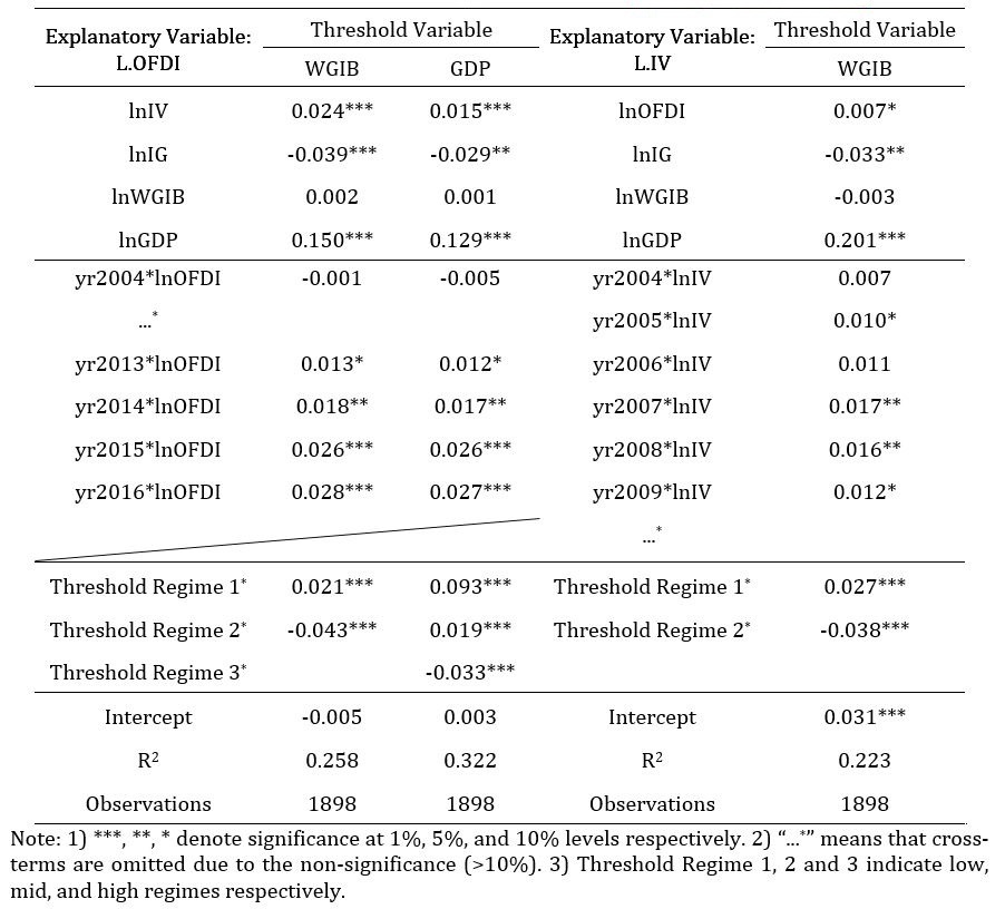
Furthermore, assessed results of the threshold regression model with fixed effects are listed in Table 4, suggesting that: 1) At higher regime of the threshold regime 1, 2 and 3 (low, mid and high, respectively), marginal growth in L.OFDI or L.IV will cut the CO2P in a statistically significant manner. For instance, at the high regime of WGIB (˃1.179) in the relationship of L.OFDI and CO2P, 1% increase in one-year lagged OFDI of China is demonstrated to lower 0.043% CO₂ emissions per capita of local country & region, of which the emissions level is noticeably less than that in the low regime. 2) When adding the cross-term combination of year dummy and OFDI or IV that is adopted to capture the time fixed effects (e.g., the impact of policies or shocks that is restricted to a set period). In the relationship of L.OFDI and CO2P, OFDI in 2014-2016 exerts an exacerbated effect on CO2P, while IV in 2007-2008 exhibits the identical effect in the relationship of L.IV and CO2P.

Table 4. Threshold regression model estimates.

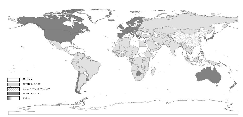
6. Verification of Threshold Variable

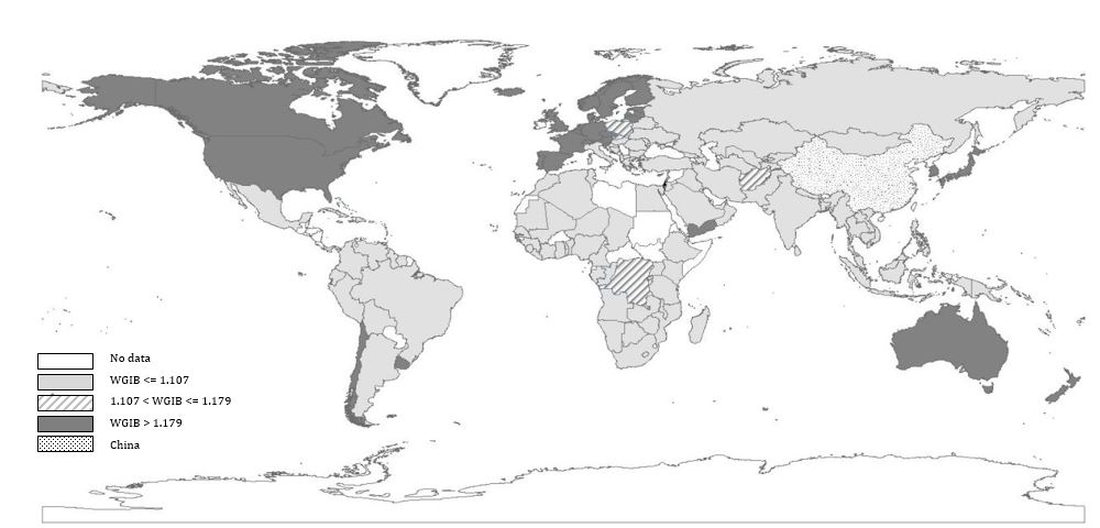
Last, to capture the spatial variability among 146 countries & regions (2003 to 2016), the threshold variable of WGIB is added into the ArcGis 10 to plot a distribution diagram at 2003 and 2016, respectively, which is statistically significant in the test of threshold effect under both relationships between L.OFDI (L.IV) and CO2P. According to Figure. 3 and 4 combined with the assessed results of Table 4, at the low regime of WGIB (<=1.107 or <=1.179), i.e., when the institutional distance between China and the specific country & region is less than 1.107 or 1.179 (high institutional proximity), the marginal increase in China’s investment or imports is demonstrated to produce 0.021% or 0.027% CO₂ emissions per capita of local areas in Asia, Africa, East Europe and South America on the whole. In contrast, at the high regime of WGIB (>1.107 or >1.179) that connects a greater institutional distance (low institutional proximity), it exerts a mitigation effect and leads to the decrease in the emission levels by 0.043% or 0.038%, when China increases its overseas investment or imports, which are intensively distributed in West & North Europe, North America, Oceania, and Northeast Asia, with a shrinking trend mainly attributed in Southeast Europe (e.g., Italy, Greece, Hungary, Slovakia, and Poland) over the years.

7. Conclusions & Suggestions

Thus far, the present study first aims to demonstrate the link between China’s rising impacts (e.g., its overseas investment and foreign trade) and economic and institutional distance with China, and CO₂ emissions per capita of 146 countries & regions (2003 to 2016). On that basis, this study aims to analyze how China’s global economic activities will impact global CO₂ emissions by exploiting the fixed effects-two stage least squares with instrumental variables. As revealed from the assessed results, increasing overseas investment from China over the years is demonstrated to exacerbate climate impacts, while China’s imports is evidently demonstrated to reduce global CO₂ emissions in the present study.

Next, the threshold regression model with fixed effects is utilized to capture how overseas investment and imports of China will impact global CO₂ emissions, at various phases of economic or institutional distance by taking it as structural breaks or threshold regimes. As a result, the marginal increase in one-year lagged OFDI or IV of China will reduce the level of global CO₂ emissions significantly at a higher threshold regime. Besides, cross-terms combined of year dummy and OFDI display significant positive correlations with CO2P in 2014-2016; cross-terms of year dummy and IV have intensified effect on CO2P in 2007-2008. Lastly, countries & regions in the low regime of WGIB (high institutional proximity) that connect with higher CO₂ emissions are primarily located in Asia, Africa, East Europe, and South America. However, the mentioned areas in the high regime of WGIB (low institutional proximity) that exert a mitigation effect on emission levels are intensively distributed in West & North Europe, North America, Oceania, and Northeast Asia, with a shrinking trend in some Southeast European countries.

In brief, the Worldwide Governance Indicators (WGI) project is determined to express the degree of the political, administrative, and legal system from the World Bank. To be specific, China is empirically likely to cut environmental effect on relatively developed markets with lower political proximity; besides, it can exert an aggravated effect on developing countries that exhibit relatively higher political proximity on the whole in overseas investment and foreign trade. Thus, given sustainability and global emissions reduction, Chinese government should keep strengthening market-oriented reform and enhancing government credibility (e.g., intellectual property, information safety, industrial subsidies, etc.), as an attempt to facilitate the political proximity with developed economies, and explore more economic cooperation with developed markets complying with a high degree of administration and environmental standards.

Explicitly speaking, China's government and multinationals are empirically encouraged to control and regulate its overextended investment in the future, and rather pay special attention to the investment quality towards the regions exerting increasing institutional proximity in recent years (e.g., a surge in economic cooperation with Southeast European countries due to the Belt & Road initiative proposed).

References

[1] G. Grossman and A. Krueger, “Economic growth and the environment,” The Quarterly Journal of Economics, vol. 110, no. 2, pp. 353-377, 1995.View Article
[2] L. Feng, “Does foreign direct investment harm the host country’s environment? Evidence from China,” SSRN Electronic Journal, 2008.
[3] G. Eskeland and A. Harrison, “Moving to greener pastures? Multinationals and the pollution haven hypothesis,” Journal of Development Economics, vol. 70, no. 1, pp. 1-23, 2003.View Article
[4] P. Grimes, J. Rey, K. Grimes and J. Kentor, “Exporting the greenhouse: Foreign capital penetration and CO2 emissions 1980–1996,” Journal of World-Systems Research, vol. 9, no. 2, pp. 261, 2003. View Article
[5] R. Hoffmann, L. C. Ging, B. Ramasamy and M. Yeung, “FDI and pollution: A Granger causality test using panel data,” Journal of International Development, vol. 17, no. 3, pp. 311-317, 2005.View Article
[6] B. Shui and R. Harriss, “The role of CO2 embodiment in US-China trade,” Energy Policy, vol. 34, no. 18, pp. 4063-4068, 2006.View Article
[7] A. Wyckoff and J. Roop, “The embodiment of carbon in imports of manufactured products: Implications for international agreements on greenhouse gas emissions,” Energy Policy, vol. 22, no. 3, pp. 187-194, 1994.View Article
[8] G. P. Peters and E. G. Hertwich, “CO2 embodied in international trade with implications for global climate policy,” Environmental science & technology, vol. 42, no. 5, pp. 1401-1407, 2008. View Article
[9] I. Kolstad and A. Wiig, “What determines Chinese outward FDI?” Journal of World Business, vol. 47, no. 1, pp. 26-34, 2012.View Article
[10] Y. W. Cheung and X. W. Qian, “Empirics of China's outward direct investment,” Pacific Economic Review, vol. 14, no. 3, pp. 312-341, 2009.View Article
[11] M. Habib and L. Zubawicki, “Corruption and foreign direct investment,” Journal of International Business Studies, vol. 33, no. 2, pp. 291-307, 2002. View Article
[12] M. Aleksynska and O. Havrylchyk, “FDI from the south: The role of institutional distance and natural resources,” European Journal of Political Economy, vol. 29, no. 284, pp. 38-53, 2013. View Article
[13] S. Lee and T. N. Sriram, “Sequential point estimation of parameters in a threshold AR(1) model,” Stochastic Processes and their Applications, vol. 84, no. 2, pp. 343-355, 1999. View Article
[14] H. Tong, “Threshold models in time series analysis— 30 years on,” Statistics and Its Interface, vol. 4, no. 2, pp. 107-118, 2011. View Article
[15] M. Mohsen and B. S. Mohsen, “The threshold impact of fiscal and monetary policies on inflation: Threshold Model Approach,” Journal of Money and Economy, vol. 10, no. 4, pp. 1-27, 2015.
[16] C. L. Chen, “The threshold effects of RMB exchange rate fluctuations on imports and exports,” Journal of Financial Risk Management, vol. 1, no. 2, pp. 15-20, 2012. View Article
[17] B. Hansen, “Threshold effects in Non-Dynamic panels: Estimation, testing, and inference,” Journal of Econometrics, vol. 93, no. 2, pp. 345-368, 1999.View Article
[18] J. Johnston, Econometric Methods. New York: McGraw-Hill, 1972.